FIN200 Assignment: Corporate Finance Management and Portfolio Theory
VerifiedAdded on 2023/06/07
|10
|2307
|405
Essay
AI Summary
This essay provides a comprehensive analysis of key concepts in corporate finance management, including the Security Market Line (SML), Capital Market Line (CML), Capital Asset Pricing Model (CAPM), and minimum variance portfolios. It differentiates between the SML and CML, highlighting their graphical representations and underlying principles. The importance of minimum variance portfolios in minimizing risk is discussed within the context of Modern Portfolio Theory (MPT). Furthermore, the essay argues for the relevance of the CAPM equation in calculating required rates of return, comparing it with the Dividend Growth Model (DGM) and Weighted Average Cost of Capital (WACC) model, and emphasizing its consideration of systematic risk. This document is a student's contribution and is available on Desklib, a platform offering study tools and resources for students.

Running head: CORPORATE FINANCE MANAGEMENT
Corporate Finance Management
Name of the Student
Name of the University
Author Note
Corporate Finance Management
Name of the Student
Name of the University
Author Note
Paraphrase This Document
Need a fresh take? Get an instant paraphrase of this document with our AI Paraphraser
1CORPORATE FINANCE MANAGEMENT
Answer to part (A)
The Security Market Line (SML) is a tool that is used to evaluate the portfolios which
is based on the Capital Asset Pricing Model. The Security Market Line establishes a
relationship between the volatility of risk and the expected returns that are associated with a
portfolio for an individual as well as the inefficient portfolios. The Security Market Line is
the main concept that is used in the Capital Asset Pricing Model. The risk that is associated
with the Security Market Line is presented in terms of beta. Beta is nothing but the security
sensitivity with regards to fluctuations in the market returns. On the other hand, Capital
Market Line is used to represent the risk free rate of return corresponding to an efficient
portfolio. The risk in case of the Capital Market Model is presented in terms of variance or
standard deviation. By standard deviation, it is meant the deviation from the mean value. The
mathematical and graphical representation of the models are provided for a better
understanding of the matter.
Let ( σ m ,rm ¿ be the point corresponding to the market portfolio M and ( σ p , r p ¿be the
point on the capital market line. The equation of the capital market line is denoted by,
r p =rf + r M −r f
σ M
σ p
Where, r p = rate of return of the efficient portfolio and σ p = variance of the expected
portfolio, rM −rf
σ M
is the price of risk as well as the slope of the Capital Market Line.
For any ith individual,
ri−rf =βi (rm−r f ) ,
Where, ri = required rate of return on the ith individual financial asset
2CORPORATE FINANCE MANAGEMENT
r f = risk free rate of return
βi = volatility of the ith individual asset
rm= average return on capital market
The above is the equation of the Security Market Line with β portfolio.
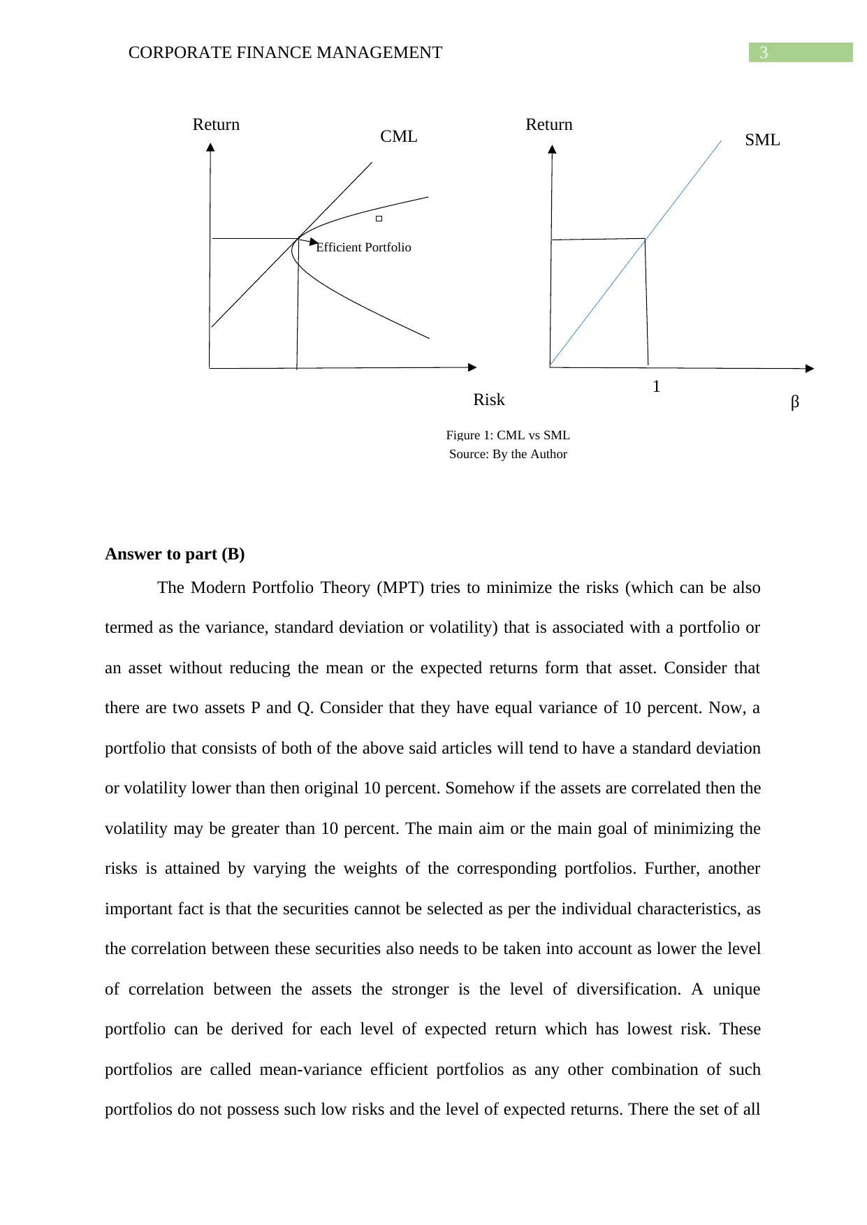
From the two diagrams provided below it can be seen that the Capital Market Line is
the locus of the point of the most efficient portfolio and the risk free rate of returns associated
with that portfolio. The tangent that passes through the efficient portfolio is the Capital Asset
Line. By efficient portfolio it is meant by the combination of the risky and risk free assets
that a person can buy which will maximize the sharp ratio. In Figure 1 the tangent passing
through the most efficient portfolio is the Capital Market Line. In contrast to that the slope of
the Security Market Line shows the volatility of the risk associated to an individual assets or
of all the portfolios which include inefficient ones. The β that is said in the above equation of
the Security Market Line is the major concern. Beta represents the measure of the changes in
security’s sensitivity with respect to that of the market returns and also the slope of the
Security Market Line. Often beta is considered as a more appropriate measure for the security
risk.
r f = risk free rate of return
βi = volatility of the ith individual asset
rm= average return on capital market
The above is the equation of the Security Market Line with β portfolio.
From the two diagrams provided below it can be seen that the Capital Market Line is
the locus of the point of the most efficient portfolio and the risk free rate of returns associated
with that portfolio. The tangent that passes through the efficient portfolio is the Capital Asset
Line. By efficient portfolio it is meant by the combination of the risky and risk free assets
that a person can buy which will maximize the sharp ratio. In Figure 1 the tangent passing
through the most efficient portfolio is the Capital Market Line. In contrast to that the slope of
the Security Market Line shows the volatility of the risk associated to an individual assets or
of all the portfolios which include inefficient ones. The β that is said in the above equation of
the Security Market Line is the major concern. Beta represents the measure of the changes in
security’s sensitivity with respect to that of the market returns and also the slope of the
Security Market Line. Often beta is considered as a more appropriate measure for the security
risk.
⊘ This is a preview!⊘
Do you want full access?
Subscribe today to unlock all pages.
Trusted by 1+ million students worldwide
3CORPORATE FINANCE MANAGEMENT
Return Return
Risk β
CML
Efficient Portfolio
1
SML
Figure 1: CML vs SML
Source: By the Author
Answer to part (B)
The Modern Portfolio Theory (MPT) tries to minimize the risks (which can be also
termed as the variance, standard deviation or volatility) that is associated with a portfolio or
an asset without reducing the mean or the expected returns form that asset. Consider that
there are two assets P and Q. Consider that they have equal variance of 10 percent. Now, a
portfolio that consists of both of the above said articles will tend to have a standard deviation
or volatility lower than then original 10 percent. Somehow if the assets are correlated then the
volatility may be greater than 10 percent. The main aim or the main goal of minimizing the
risks is attained by varying the weights of the corresponding portfolios. Further, another
important fact is that the securities cannot be selected as per the individual characteristics, as
the correlation between these securities also needs to be taken into account as lower the level
of correlation between the assets the stronger is the level of diversification. A unique
portfolio can be derived for each level of expected return which has lowest risk. These
portfolios are called mean-variance efficient portfolios as any other combination of such
portfolios do not possess such low risks and the level of expected returns. There the set of all
Paraphrase This Document
Need a fresh take? Get an instant paraphrase of this document with our AI Paraphraser
4CORPORATE FINANCE MANAGEMENT
Returns
Risks
Minimum Variance Portfolio
Efficient Frontier
Individual Securities
Figure 2: Efficient Frontier
S
Source
R1 R2 R3
Source: By the Author
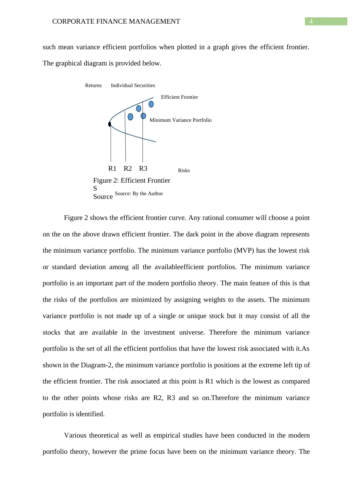
such mean variance efficient portfolios when plotted in a graph gives the efficient frontier.
The graphical diagram is provided below.
Figure 2 shows the efficient frontier curve. Any rational consumer will choose a point
on the on the above drawn efficient frontier. The dark point in the above diagram represents
the minimum variance portfolio. The minimum variance portfolio (MVP) has the lowest risk
or standard deviation among all the availableefficient portfolios. The minimum variance
portfolio is an important part of the modern portfolio theory. The main feature of this is that
the risks of the portfolios are minimized by assigning weights to the assets. The minimum
variance portfolio is not made up of a single or unique stock but it may consist of all the
stocks that are available in the investment universe. Therefore the minimum variance
portfolio is the set of all the efficient portfolios that have the lowest risk associated with it.As
shown in the Diagram-2, the minimum variance portfolio is positions at the extreme left tip of
the efficient frontier. The risk associated at this point is R1 which is the lowest as compared
to the other points whose risks are R2, R3 and so on.Therefore the minimum variance
portfolio is identified.
Various theoretical as well as empirical studies have been conducted in the modern
portfolio theory, however the prime focus have been on the minimum variance theory. The
Returns
Risks
Minimum Variance Portfolio
Efficient Frontier
Individual Securities
Figure 2: Efficient Frontier
S
Source
R1 R2 R3
Source: By the Author
such mean variance efficient portfolios when plotted in a graph gives the efficient frontier.
The graphical diagram is provided below.
Figure 2 shows the efficient frontier curve. Any rational consumer will choose a point
on the on the above drawn efficient frontier. The dark point in the above diagram represents
the minimum variance portfolio. The minimum variance portfolio (MVP) has the lowest risk
or standard deviation among all the availableefficient portfolios. The minimum variance
portfolio is an important part of the modern portfolio theory. The main feature of this is that
the risks of the portfolios are minimized by assigning weights to the assets. The minimum
variance portfolio is not made up of a single or unique stock but it may consist of all the
stocks that are available in the investment universe. Therefore the minimum variance
portfolio is the set of all the efficient portfolios that have the lowest risk associated with it.As
shown in the Diagram-2, the minimum variance portfolio is positions at the extreme left tip of
the efficient frontier. The risk associated at this point is R1 which is the lowest as compared
to the other points whose risks are R2, R3 and so on.Therefore the minimum variance
portfolio is identified.
Various theoretical as well as empirical studies have been conducted in the modern
portfolio theory, however the prime focus have been on the minimum variance theory. The
5CORPORATE FINANCE MANAGEMENT
importance of the minimum variance portfolio can be described as follows. There exists a
large number of companies who are running their investment funds strategy that are solely
based on the minimum variance optimization. Further, the minimum variance theory has also
drawn attention of the stock exchange. The index providers are also benefited from the
minimum variance theory. There exists three reasons for the prevalence of the minimum
variance portfolio. Firstly most of the empirical studies that has been conducted till date
shows that the minimum variance portfolio has performed relatively well than any other
indexes. Secondly, when the optimization is conducted, the optimization of minimum
variance portfolio does not require considering the expected returns forecasts. In other words
the optimization is independent from the expected returns forecast. These expected returns
forecast are the major source of errors that arise due to estimation. Lastly, it has been seen
that the participant in the market are primarily risk averse in nature. This phenomenon
stimulates the creation of the financial products with a managed volatility. In this case the
minimum variance theory serves to the needs of the investors.
Answer to part (C)
The Capital Asset Pricing Model (CAPM) establishes a linear relationship between
the required rates of return and the systematic risk associated with that investment. This
investment might be in the form stock market securities or in the form of business operation.
The Capital Asset Pricing Model incorporates the Security Market Line concept. The general
equation of the model is,
ri−rf =βi (rm−r f )
ri=rf + βi (r m−r f )
Where, ri = required rate of return on the ith individual financial asset
r f = risk free rate of return
⊘ This is a preview!⊘
Do you want full access?
Subscribe today to unlock all pages.
Trusted by 1+ million students worldwide
6CORPORATE FINANCE MANAGEMENT
βi = volatility of the ith individual asset
rm= average return on capital market
The Capital Asset Model has an upper advantage and is more relevant than any other
equation while calculating the required rate of return. While calculating the rate of return the
Capital Asset Pricing Model model considers only the systematic risk. The systematic risks
are those risks that cannot be diversified. These systematic risks are caused due to external
factors occurring to an organisation. These risks cannot be controlled by nature. The beta that
is used in the Capital Asset Pricing Model takes into account these systematic risks. In any
other model these are not included. This fact is quite realistic as most of the investors have a
diversified portfolio and the unsystematic risks associated with these portfolios are essentially
eliminated. Another factor that can be stated relating to the relevance of the Capital Asset
Pricing Model equation is that the model generates a theoretical relationship between the
required return rates and the systematic risks associated with the assets which is a matter of
frequent discussion. The equation when implied in real life scenario has a great relevance.
The Dividend Growth Model (DGM) that also tries to calculate the return rates but, the
Capital Asset Pricing Model is far more superior. The Dividend Growth Model assumes that
the rate of growth of dividends is constant in perpetuity. The value of the stock is equal to the
following year’s dividends divided by difference between the required rate of return and the
constant growth rate in dividends that is assumed (McKenzie and Partington 2013).the model
is further divided into two categories the stable model and the multistage growth model. The
equation for the stable model can be represented as follows:
P= d1
k −g , where, P = value of stock, d1 is the next year’s dividends, k = rate of return
and g is the constant rate of growth. The Dividend Growth Model explicitly takes into
account the company’s level of the systematic risks relative to that of the stock as a whole.
Paraphrase This Document
Need a fresh take? Get an instant paraphrase of this document with our AI Paraphraser
7CORPORATE FINANCE MANAGEMENT
B
A
C
SML
WACC
Risk
β
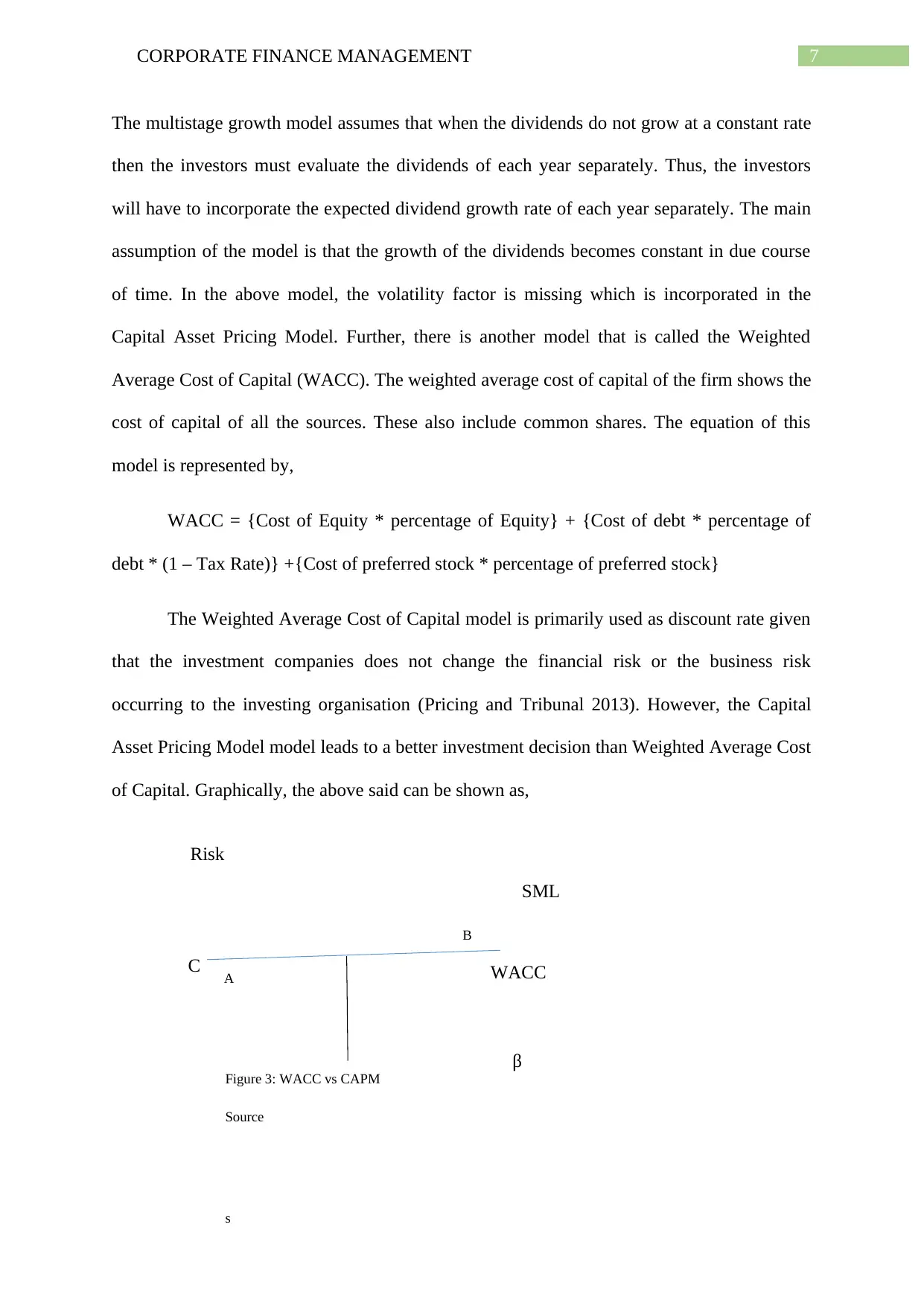
Figure 3: WACC vs CAPM
Source
s
The multistage growth model assumes that when the dividends do not grow at a constant rate
then the investors must evaluate the dividends of each year separately. Thus, the investors
will have to incorporate the expected dividend growth rate of each year separately. The main
assumption of the model is that the growth of the dividends becomes constant in due course
of time. In the above model, the volatility factor is missing which is incorporated in the
Capital Asset Pricing Model. Further, there is another model that is called the Weighted
Average Cost of Capital (WACC). The weighted average cost of capital of the firm shows the
cost of capital of all the sources. These also include common shares. The equation of this
model is represented by,
WACC = {Cost of Equity * percentage of Equity} + {Cost of debt * percentage of
debt * (1 – Tax Rate)} +{Cost of preferred stock * percentage of preferred stock}
The Weighted Average Cost of Capital model is primarily used as discount rate given
that the investment companies does not change the financial risk or the business risk
occurring to the investing organisation (Pricing and Tribunal 2013). However, the Capital
Asset Pricing Model model leads to a better investment decision than Weighted Average Cost
of Capital. Graphically, the above said can be shown as,
B
A
C
SML
WACC
Risk
β
Figure 3: WACC vs CAPM
Source
s
The multistage growth model assumes that when the dividends do not grow at a constant rate
then the investors must evaluate the dividends of each year separately. Thus, the investors
will have to incorporate the expected dividend growth rate of each year separately. The main
assumption of the model is that the growth of the dividends becomes constant in due course
of time. In the above model, the volatility factor is missing which is incorporated in the
Capital Asset Pricing Model. Further, there is another model that is called the Weighted
Average Cost of Capital (WACC). The weighted average cost of capital of the firm shows the
cost of capital of all the sources. These also include common shares. The equation of this
model is represented by,
WACC = {Cost of Equity * percentage of Equity} + {Cost of debt * percentage of
debt * (1 – Tax Rate)} +{Cost of preferred stock * percentage of preferred stock}
The Weighted Average Cost of Capital model is primarily used as discount rate given
that the investment companies does not change the financial risk or the business risk
occurring to the investing organisation (Pricing and Tribunal 2013). However, the Capital
Asset Pricing Model model leads to a better investment decision than Weighted Average Cost
of Capital. Graphically, the above said can be shown as,
8CORPORATE FINANCE MANAGEMENT
From the diagram, point A is not feasible in case of Weighted Average Cost of
Capital as the internal rate of return is less than the Weighted Average Cost of Capital
intercept C whereas if Capital Asset Pricing Model would have been considered then, A
would have been a feasible option. Similarly, for point B, it would have been feasible for
Weighted Average Cost of Capital. The point B is has a rate of return much higher than the
internal rate of return. Thus, considering the Weighted Average Cost of Capital model this
point B would have been feasible. However, when Capital Asset Pricing Model is considered
then this point is not all a feasible point. Point B provides insufficient compensations for the
level of systematic risks. There it can be clearly how the Capital Asset Pricing Model is far
superior than any of the existing theories.
⊘ This is a preview!⊘
Do you want full access?
Subscribe today to unlock all pages.
Trusted by 1+ million students worldwide

9CORPORATE FINANCE MANAGEMENT
Reference
McKenzie, M. and Partington, G., 2013. The dividend growth model (DGM). Report to the
AER.
Pricing, I. and Tribunal, R., 2013. Review of WACC methodology. Research–Final report.
Reference
McKenzie, M. and Partington, G., 2013. The dividend growth model (DGM). Report to the
AER.
Pricing, I. and Tribunal, R., 2013. Review of WACC methodology. Research–Final report.
1 out of 10
Related Documents


Your All-in-One AI-Powered Toolkit for Academic Success.
+13062052269
info@desklib.com
Available 24*7 on WhatsApp / Email
![[object Object]](/_next/static/media/star-bottom.7253800d.svg)
Unlock your academic potential
Copyright © 2020–2026 A2Z Services. All Rights Reserved. Developed and managed by ZUCOL.