Impact of Income and Household Size on Credit Card Spending Analysis

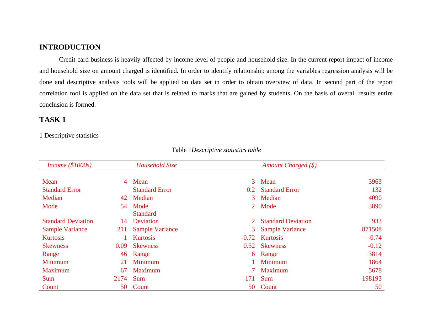
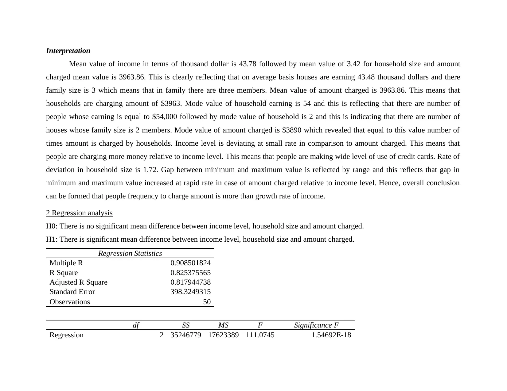
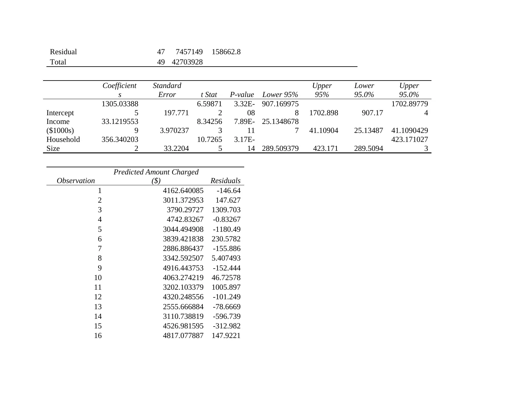
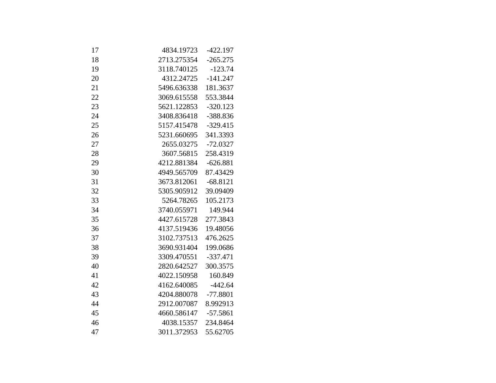
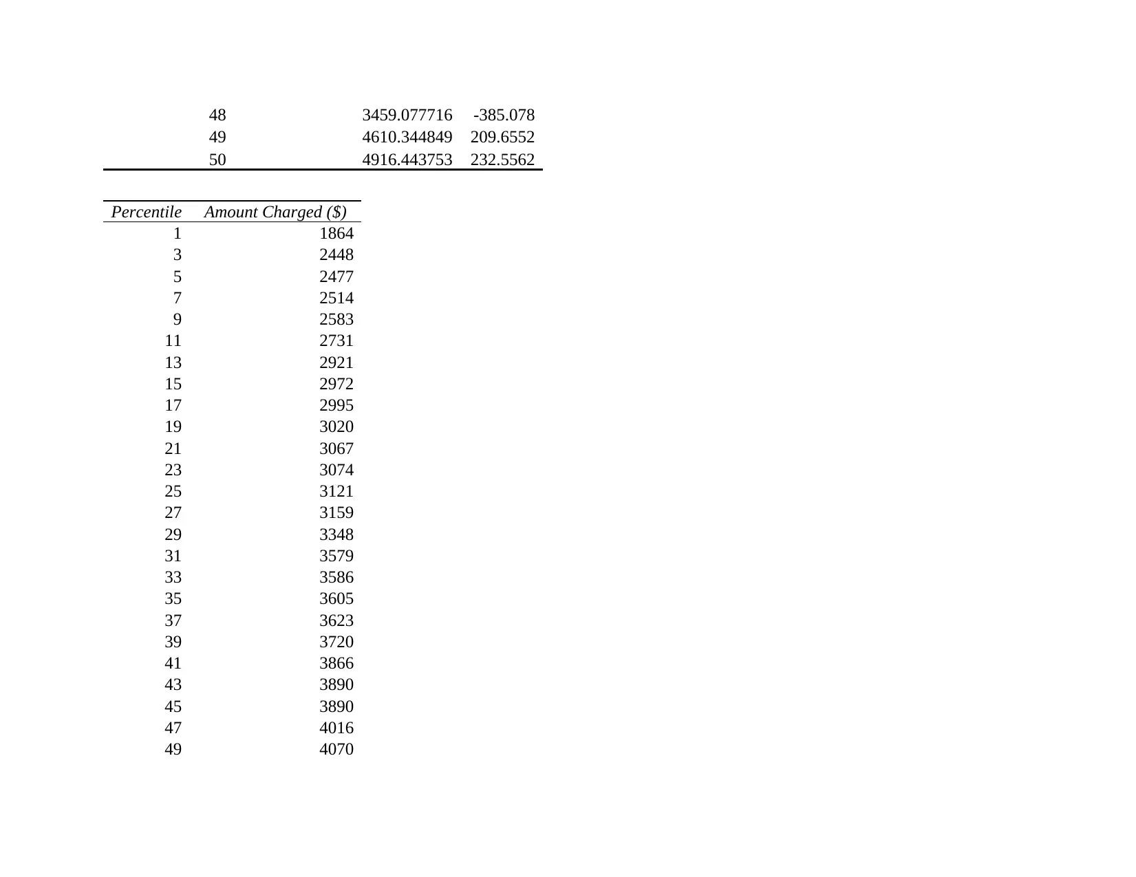
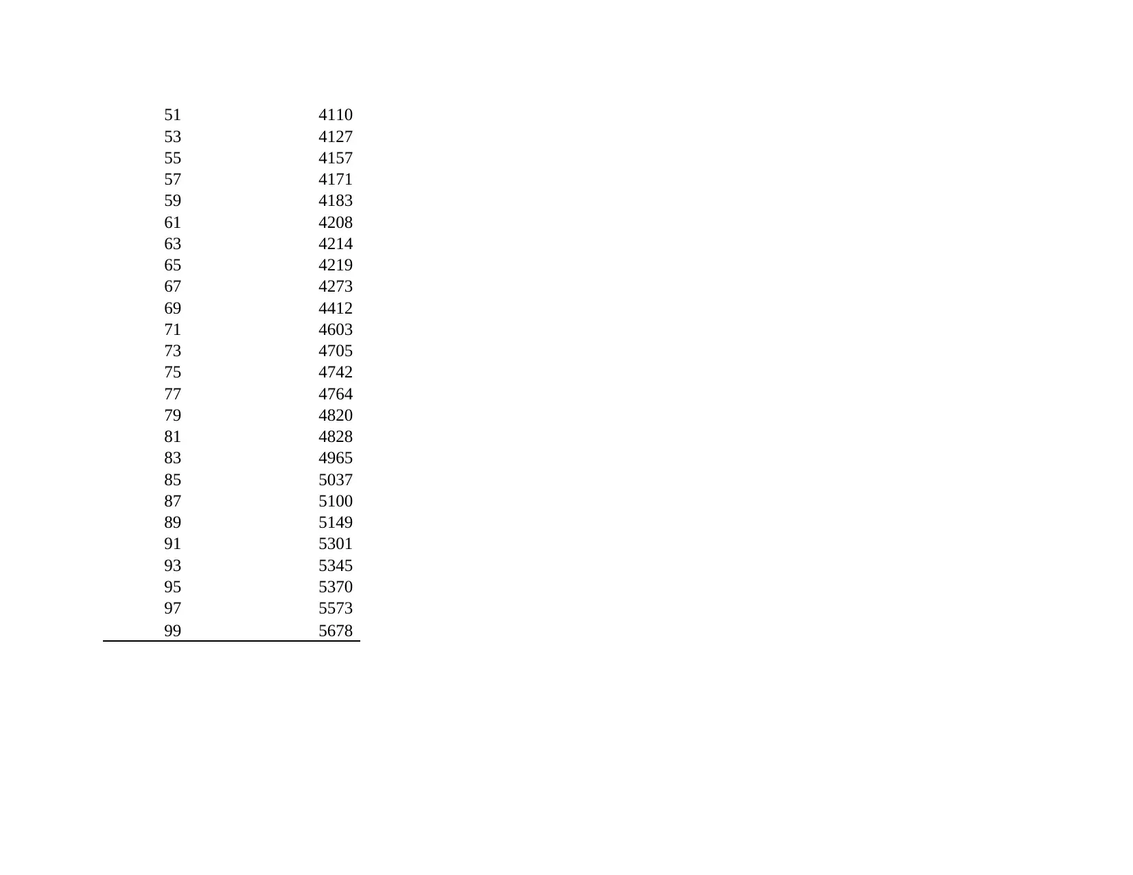
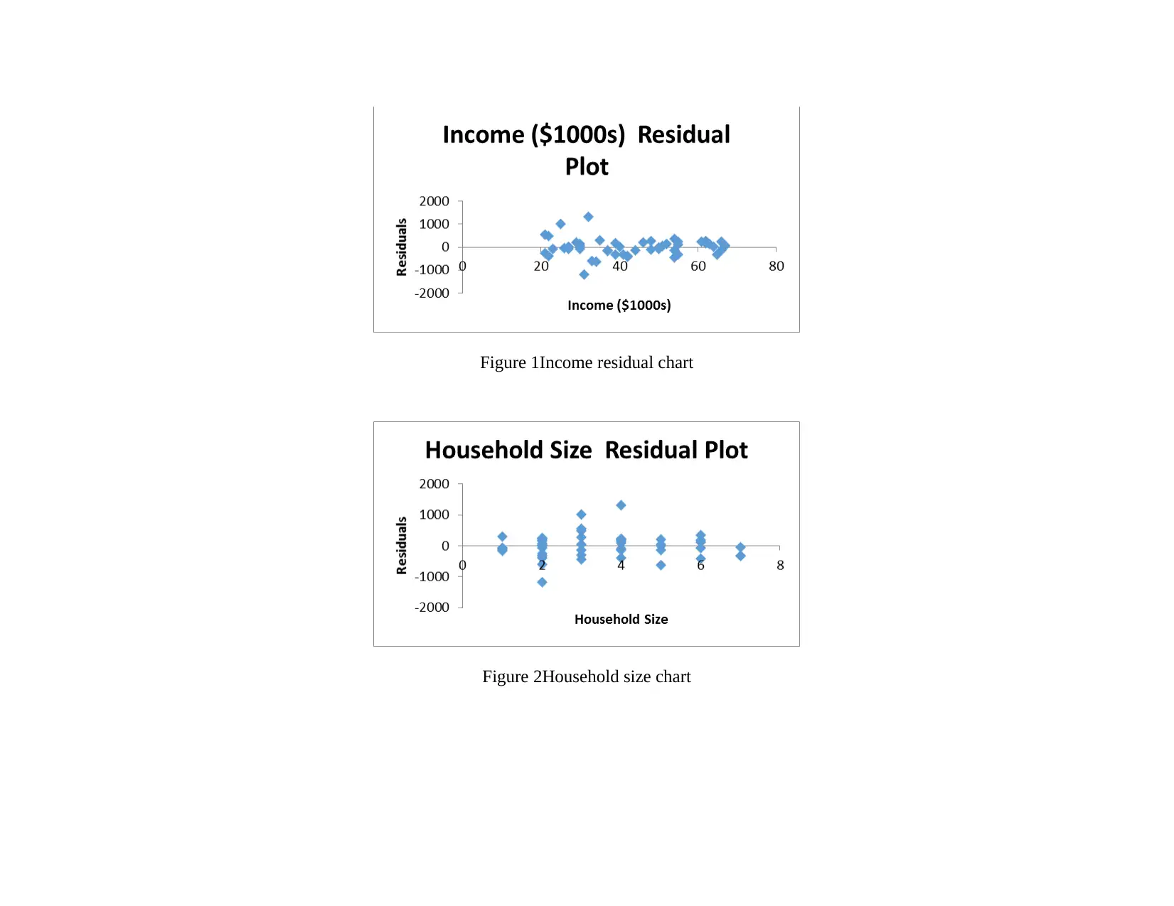
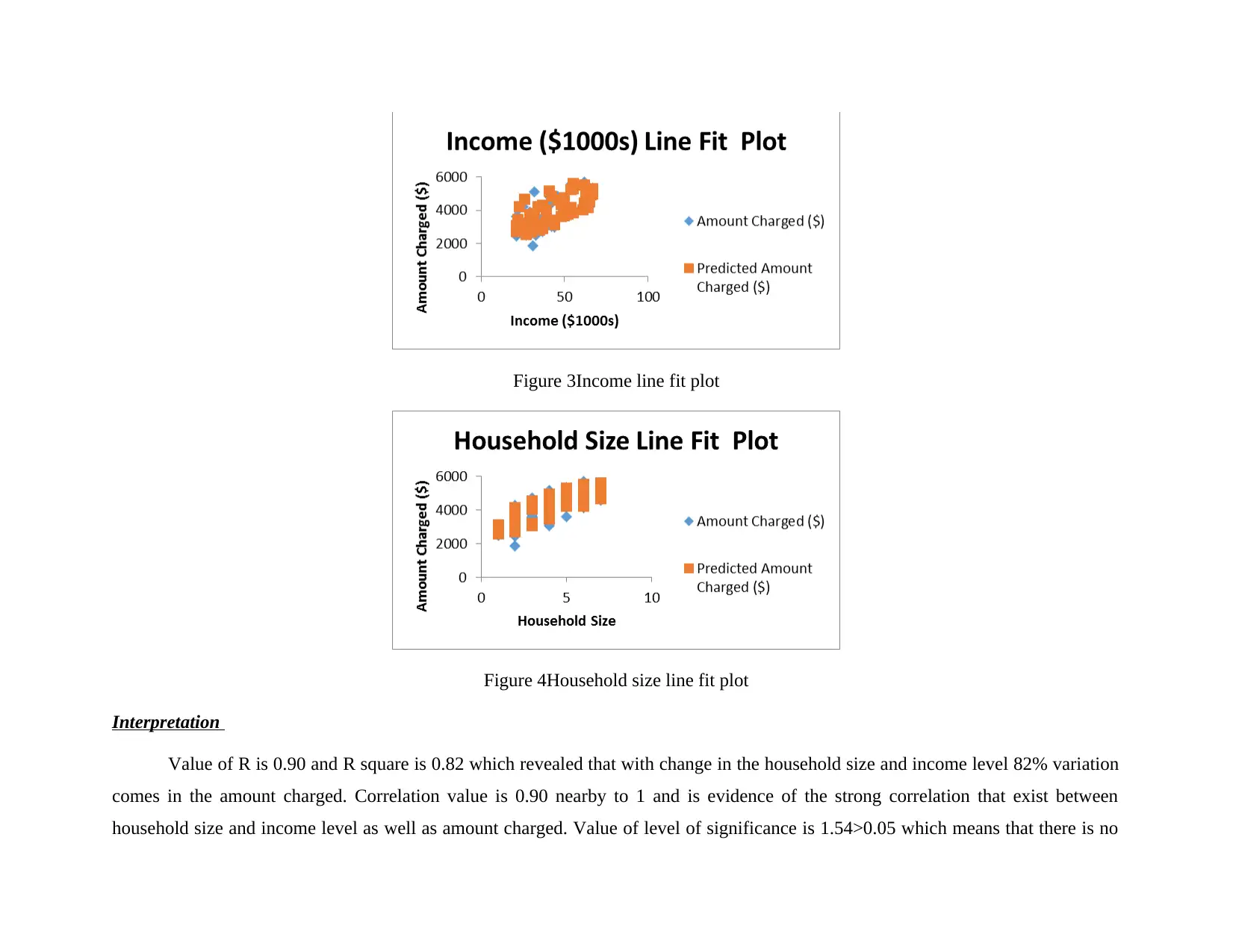
This report investigates the relationship between income, household size, and credit card spending using descriptive statistics and regression analysis. The analysis reveals a strong correlation between household size, income levels, and the amount charged on credit cards. The descriptive statistics provide an overview of the data, while the regression analysis identifies the impact of income and household size on spending. The study predicts average spending for a household size of three with an annual income of $40,000. The report also includes an analysis of student marks, applying correlation tools to assess relationships between different assessment components. The findings suggest that changes in household size have a more significant impact on credit card charges than income levels. The report concludes with an overall assessment of the variables, and suggests further analysis by introducing additional independent variables.

STATISTICS BUSINESS DECISION

TABLE OF CONTENT
INTRODUCTION.......................................................................................................................................................................................3
TASK 1........................................................................................................................................................................................................3
1 Descriptive statistics.............................................................................................................................................................................3
2 Regression analysis...............................................................................................................................................................................4
3 Regression equation for both independent and dependent variable...................................................................................................11
4 Predicted charge in case household size is three person with annual income level of $40000..........................................................11
5 Addition of variables..........................................................................................................................................................................11
TASK 2......................................................................................................................................................................................................12
Activity 01.............................................................................................................................................................................................12
Activity 02.............................................................................................................................................................................................12
Activity 03.............................................................................................................................................................................................23
CONCLUSION..........................................................................................................................................................................................29

INTRODUCTION
Credit card business is heavily affected by income level of people and household size. In the current report impact of income
and household size on amount charged is identified. In order to identify relationship among the variables regression analysis will be
done and descriptive analysis tools will be applied on data set in order to obtain overview of data. In second part of the report
correlation tool is applied on the data set that is related to marks that are gained by students. On the basis of overall results entire
conclusion is formed.
TASK 1
1 Descriptive statistics
Table 1Descriptive statistics table
Income ($1000s) Household Size Amount Charged ($)
Mean 4 Mean 3 Mean 3963
Standard Error Standard Error 0.2 Standard Error 132
Median 42 Median 3 Median 4090
Mode 54 Mode 2 Mode 3890
Standard Deviation 14
Standard
Deviation 2 Standard Deviation 933
Sample Variance 211 Sample Variance 3 Sample Variance 871508
Kurtosis -1 Kurtosis -0.72 Kurtosis -0.74
Skewness 0.09 Skewness 0.52 Skewness -0.12
Range 46 Range 6 Range 3814
Minimum 21 Minimum 1 Minimum 1864
Maximum 67 Maximum 7 Maximum 5678
Sum 2174 Sum 171 Sum 198193
Count 50 Count 50 Count 50

Interpretation
Mean value of income in terms of thousand dollar is 43.78 followed by mean value of 3.42 for household size and amount
charged mean value is 3963.86. This is clearly reflecting that on average basis houses are earning 43.48 thousand dollars and there
family size is 3 which means that in family there are three members. Mean value of amount charged is 3963.86. This means that
households are charging amount of $3963. Mode value of household earning is 54 and this is reflecting that there are number of
people whose earning is equal to $54,000 followed by mode value of household is 2 and this is indicating that there are number of
houses whose family size is 2 members. Mode value of amount charged is $3890 which revealed that equal to this value number of
times amount is charged by households. Income level is deviating at small rate in comparison to amount charged. This means that
people are charging more money relative to income level. This means that people are making wide level of use of credit cards. Rate of
deviation in household size is 1.72. Gap between minimum and maximum value is reflected by range and this reflects that gap in
minimum and maximum value increased at rapid rate in case of amount charged relative to income level. Hence, overall conclusion
can be formed that people frequency to charge amount is more than growth rate of income.
2 Regression analysis
H0: There is no significant mean difference between income level, household size and amount charged.
H1: There is significant mean difference between income level, household size and amount charged.
Regression Statistics
Multiple R 0.908501824
R Square 0.825375565
Adjusted R Square 0.817944738
Standard Error 398.3249315
Observations 50
df SS MS F Significance F
Regression 2 35246779 17623389 111.0745 1.54692E-18

Residual 47 7457149 158662.8
Total 49 42703928
Coefficient
s
Standard
Error t Stat P-value Lower 95%
Upper
95%
Lower
95.0%
Upper
95.0%
Intercept
1305.03388
5 197.771
6.59871
2
3.32E-
08
907.169975
8 1702.898 907.17
1702.89779
4
Income
($1000s)
33.1219553
9 3.970237
8.34256
3
7.89E-
11
25.1348678
7 41.10904 25.13487 41.1090429
Household
Size
356.340203
2 33.2204
10.7265
5
3.17E-
14 289.509379 423.171 289.5094
423.171027
3
Observation
Predicted Amount Charged
($) Residuals
1 4162.640085 -146.64
2 3011.372953 147.627
3 3790.29727 1309.703
4 4742.83267 -0.83267
5 3044.494908 -1180.49
6 3839.421838 230.5782
7 2886.886437 -155.886
8 3342.592507 5.407493
9 4916.443753 -152.444
10 4063.274219 46.72578
11 3202.103379 1005.897
12 4320.248556 -101.249
13 2555.666884 -78.6669
14 3110.738819 -596.739
15 4526.981595 -312.982
16 4817.077887 147.9221

17 4834.19723 -422.197
18 2713.275354 -265.275
19 3118.740125 -123.74
20 4312.24725 -141.247
21 5496.636338 181.3637
22 3069.615558 553.3844
23 5621.122853 -320.123
24 3408.836418 -388.836
25 5157.415478 -329.415
26 5231.660695 341.3393
27 2655.03275 -72.0327
28 3607.56815 258.4319
29 4212.881384 -626.881
30 4949.565709 87.43429
31 3673.812061 -68.8121
32 5305.905912 39.09409
33 5264.78265 105.2173
34 3740.055971 149.944
35 4427.615728 277.3843
36 4137.519436 19.48056
37 3102.737513 476.2625
38 3690.931404 199.0686
39 3309.470551 -337.471
40 2820.642527 300.3575
41 4022.150958 160.849
42 4162.640085 -442.64
43 4204.880078 -77.8801
44 2912.007087 8.992913
45 4660.586147 -57.5861
46 4038.15357 234.8464
47 3011.372953 55.62705

48 3459.077716 -385.078
49 4610.344849 209.6552
50 4916.443753 232.5562
Percentile Amount Charged ($)
1 1864
3 2448
5 2477
7 2514
9 2583
11 2731
13 2921
15 2972
17 2995
19 3020
21 3067
23 3074
25 3121
27 3159
29 3348
31 3579
33 3586
35 3605
37 3623
39 3720
41 3866
43 3890
45 3890
47 4016
49 4070

51 4110
53 4127
55 4157
57 4171
59 4183
61 4208
63 4214
65 4219
67 4273
69 4412
71 4603
73 4705
75 4742
77 4764
79 4820
81 4828
83 4965
85 5037
87 5100
89 5149
91 5301
93 5345
95 5370
97 5573
99 5678

Figure 1Income residual chart
Figure 2Household size chart

Figure 3Income line fit plot
Figure 4Household size line fit plot
Interpretation
Value of R is 0.90 and R square is 0.82 which revealed that with change in the household size and income level 82% variation
comes in the amount charged. Correlation value is 0.90 nearby to 1 and is evidence of the strong correlation that exist between
household size and income level as well as amount charged. Value of level of significance is 1.54>0.05 which means that there is no

significant difference between mean values of the independent and dependent variable. It can be interpreted that rate of change in
independent and dependent variable is same. It can be interpreted that rate at which household size and income level changed at same
rate people spending get changed. Thus, null hypothesis is accepted.
3 Regression equation for both independent and dependent variable
Income level= a+ bx
=1305+33.12*x
Household size= a+bx
= 1305+356*x
On analysis of figures it is clearly observed that there is no significant mean difference in terms of rate of change that is observed in
case of income level and household size. Means that rate of change in amount charge is high but that change is not too high relative to
variables income level and household size. It can be said that household size heavily affect dependent variable in comparison to
income level. Thus, it can be said that in case elevation is observed in household size then amount charged may vary to great extent.
4 Predicted charge in case household size is three person with annual income level of $40000
Household size= a+ bx
= 1305+356*3=2373
Average spend will be $2373 in case any family size will be three person and income level is $40000.
5 Addition of variables
As part of addition of new independent variable household saving rate can also be taken in to consideration and change that
comes in amount charged in respect to household saving can be identified by using regression analysis tools.

TASK 2
Activity 01
Data are arranged in variable view in excel sheet.
Activity 02
(a)Drawing histogram
Figure 5HI001 Final exam

Figure 6HI001 assignment 1
Figure 7HI001 assignment 02

Figure 8HI002 final exam
Figure 9HI002 assignment 01

Figure 10HI002 assignment 02
Figure 11HI003 final exam

Figure 12HI003 assignment 01
Figure 13HI003 assignment 02
(b)Descriptive statistics

Student
ID Year
Enrolled
HI001
FINAL
EXAM
HI001
ASSIGNMEN
T 01
HI001
ASSIGNMEN
T 02
HI002
FINAL
EXAM
HI002
ASSIGNMEN
T 01
HI002
ASSIGNMEN
T 02
HI003
FINAL
EXAM
Mean 2013.04 32.39 17.21 15.46 26.77 17.82 12.42 25.99
STDEV 0.81124
4.99551
3 1.990959 2.31164
5.28264
7 3.44125 1.989267
8.27179
4
MIN 2012.00 20.00 8.00 8.00 12.00 4.00 4.00 4.00
MAX 2014.00 45.00 22.00 21.00 40.00 22.00 16.00 43.00
18.19 13.54 49.50
3.907851 1.759618 28.43413442
10.00 8.00 1.00
30.00 20.00 98.00
Interpretation
In case of HI001 final exam mean value of score is 32.99 and same in case of HI002 is 17.82 followed by HI003 is 25.99. This
means that more marks are earned in first and third test. Standard deviation for HI001 is 4.99 and same for HI002 is 5.28 followed by
HI003 is 8.27. Results are clearly reflecting that marks are deviating at higher rate in case of HI003 exam then compared one. Gap
between maximum and minimum value is high in case of HI003 final exam relative to compared one. It can be said that students are
earning higher marks in case of HI003 then HI001 and HI002.
Activity 03
HI001Finalexam HI001Assignment01 HI001Assignment02 HI002Finalexam HI002Assignment01
HI001Finalexam Pearson
Correlation
1 .093 .342** .049 -.002
Sig. (2- .364 .001 .630 .986

tailed)
N 98 98 98 98 98
HI001Assignment01 Pearson
Correlation
.093 1 .659** -.015 -.131
Sig. (2-
tailed)
.364 .000 .881 .198
N 98 98 98 98 98
HI001Assignment02 Pearson
Correlation
.342** .659** 1 -.037 -.097
Sig. (2-
tailed)
.001 .000 .715 .343
N 98 98 98 98 98
HI002Finalexam Pearson
Correlation
.049 -.015 -.037 1 .177
Sig. (2-
tailed)
.630 .881 .715 .081
N 98 98 98 98 98
HI002Assignment01 Pearson
Correlation
-.002 -.131 -.097 .177 1
Sig. (2-
tailed)
.986 .198 .343 .081
N 98 98 98 98 98
HI002Assignment02 Pearson
Correlation
-.034 -.093 -.038 .363** .549**
Sig. (2-
tailed)
.743 .362 .712 .000 .000
N 98 98 98 98 98
HI003Finalexam Pearson
Correlation
.122 .232* .277** .116 .016

Sig. (2-
tailed)
.232 .022 .006 .257 .880
N 98 98 98 98 98
HI003Assignment01 Pearson
Correlation
-.044 -.004 .049 -.060 -.232*
Sig. (2-
tailed)
.670 .968 .629 .557 .022
N 98 98 98 98 98
HI003Assignment02 Pearson
Correlation
.219* .096 .101 -.074 -.155
Sig. (2-
tailed)
.030 .347 .325 .470 .127
N 98 98 98 98 98
Studentcoding Pearson
Correlation
-.267** .020 -.152 -.080 -.199*
Sig. (2-
tailed)
.008 .845 .135 .436 .049
N 98 98 98 98 98
HI002Assignment02 HI003Finalexam HI003Assignment01 HI003Assignment02 Studentcoding
HI001Finalexam Pearson
Correlation
-.034 .122 -.044 .219* -.267**
Sig. (2-
tailed)
.743 .232 .670 .030 .008
N 98 98 98 98 98

HI001Assignment01 Pearson
Correlation
-.093 .232* -.004 .096 .020
Sig. (2-
tailed)
.362 .022 .968 .347 .845
N 98 98 98 98 98
HI001Assignment02 Pearson
Correlation
-.038 .277** .049 .101 -.152
Sig. (2-
tailed)
.712 .006 .629 .325 .135
N 98 98 98 98 98
HI002Finalexam Pearson
Correlation
.363** .116 -.060 -.074 -.080
Sig. (2-
tailed)
.000 .257 .557 .470 .436
N 98 98 98 98 98
HI002Assignment01 Pearson
Correlation
.549** .016 -.232* -.155 -.199*
Sig. (2-
tailed)
.000 .880 .022 .127 .049
N 98 98 98 98 98
HI002Assignment02 Pearson
Correlation
1 .164 -.192 -.107 -.161
Sig. (2-
tailed)
.107 .058 .296 .113
N 98 98 98 98 98
HI003Finalexam Pearson
Correlation
.164 1 .197 .120 .067
Sig. (2-
tailed)
.107 .052 .239 .515

N 98 98 98 98 98
HI003Assignment01 Pearson
Correlation
-.192 .197 1 .520** .240*
Sig. (2-
tailed)
.058 .052 .000 .017
N 98 98 98 98 98
HI003Assignment02 Pearson
Correlation
-.107 .120 .520** 1 -.121
Sig. (2-
tailed)
.296 .239 .000 .233
N 98 98 98 98 98
Studentcoding Pearson
Correlation
-.161 .067 .240* -.121 1
Sig. (2-
tailed)
.113 .515 .017 .233
N 98 98 98 98 98
Interpretation
 HI001 final exam: HI001correlation value is moderate in case of HI001 assignment 02 and HI003 assignment 02.
Correlations are positively related and level of significance value for both variables is 0.01<0.05 and 0.03<0.05. This reflect
that there is significant relationship between both variables. It can be said that with change in marks gained on HI001 final
exam marks earned on HI001 assignment 02 and HI003 assignment 02 get influenced. In case of other variables there is low
correlation value and there is significant relationship among variables. However, negative and low correlation is observed in
case of HI002 assignment 02 and HI003 assignment 01. It can be said that second assignment of HI002 and first assignment of
HI003 are negatively influenced by the HI001 final exam marks.

 H1001 assignment 01: Mentioned variable have high correlation with HI001 assignment 2 0.65(0.00<0.05), low correlation
with HI003 final exam 0.232(0.02<0.05). On other hand, low correlation value is observed in case of HI002 final exam -
0.15(0.881>0.05), HI002 assignment 1 -0.97(0.343>0.5). It can be said that results of HI001 are directly positively related with
HI001 assignment and HI003 final exam.
 HI001 assignment 02: Moderate correlation is identified in case of HI003 final exam 0.277(0.06>0.05) and HI003 assignment
1 0.049 (0.629>0.05). Apart from this, in case of all other variables there is negative correlation between variables. It can be
said that HI001 assignment 2 have positive impact on HI003 final exam and HI003 assignment 1.
 HI002 final exam: Positive correlation is observed in case of HI002 assignment 1 0.177(0.081>0.05), HI002 assignment 2
0.363(0.00>0.05), HI003 final exam 0.116(0.257>0.05). Results are clearly reflecting that there is high correlation between
HI002 final exam and HI002 assignment 2 and have moderate or low correlation with HI003 final exam. In case of HI003
assignment 1 -0.60(0.60>0.05) and HI003 assignment 02 -0.74(0.470>0.05). Hence, there is low correlation of HI002 final
exam with HI003 assignment 1 and assignment 2.
 HI002 assignment 01: Mentioned variable have positive correlation with HI002 assignment 02 0.549(0.00>0.05), HI003 final
exam 0.016(0.880>0.05). On other hand, mentioned variable have negative relationship with HI003 assignment 01 -
232(0.02<0.05), HI003 assignment 02 -0.74(0.470). It can be said that when students will gain positive marks on assignment 1
then in assignment 2 also positive marks will be gained. However, if positive marks will be gained on assignment 01 then in
that case negative marks will be gained on both assignments of HI003.
 HI002 assignment 02: HI002 assignment 02 have positive correlation with HI003 final exam 0.164(0.107>0.05). In case of
HI003 assignment 01 there is negative correlation -.192(0.05=0.05) and HI003 assignment 02 -107(0.296>0.05). This reflects
that if positive marks are gained on HI002 assignment 02 then in HI003 final exam also positive marks can be obtained but
there is no significant relationship between both. Similarly, if positive marks will be gained on HI002 assignment 02 then in
that case less number of marks can be obtained on both assignments of HI003.

 HI003 final exam: There is positive correlation of HI003 final exam with HI003 assignment 1 with 0.197(0.05=0.05) and
HI003 assignment 02 0.120(0.239>0.05). It can be said that if positive marks are obtained on both assignments then surely
good results can be observed in HI003 final exam.
 HI003 assignment 01: There is positive correlation value of HI003 assignment 01 with HI003 assignment 02 as correlation
value is 0.520 (0.00<0.05). This means that marks gained on HI003 assignment 02 is highly affected by marks that are gained
on HI003 assignment 01.
CONCLUSION
On the basis of above discussion it can be concluded that assignments results does not have strong influence on the marks that
are obtained on the final exam. However, to some extent assignments have interrelation with each other in terms of marks that are
obtained by the students. It can be said that even in one assignment one gained high marks then it does not mean that same person will
gain higher marks on other assignments or final exams. It is also concluded that there significant mean difference between variables
income and household size in terms of impact that both have on the amount charged. It can be said that both independent variables
have equal impact on dependent variable which is amount charged.