Comprehensive Statistical Analysis Report: Credit Card Data

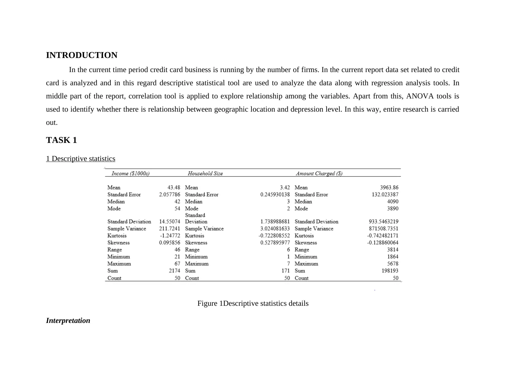
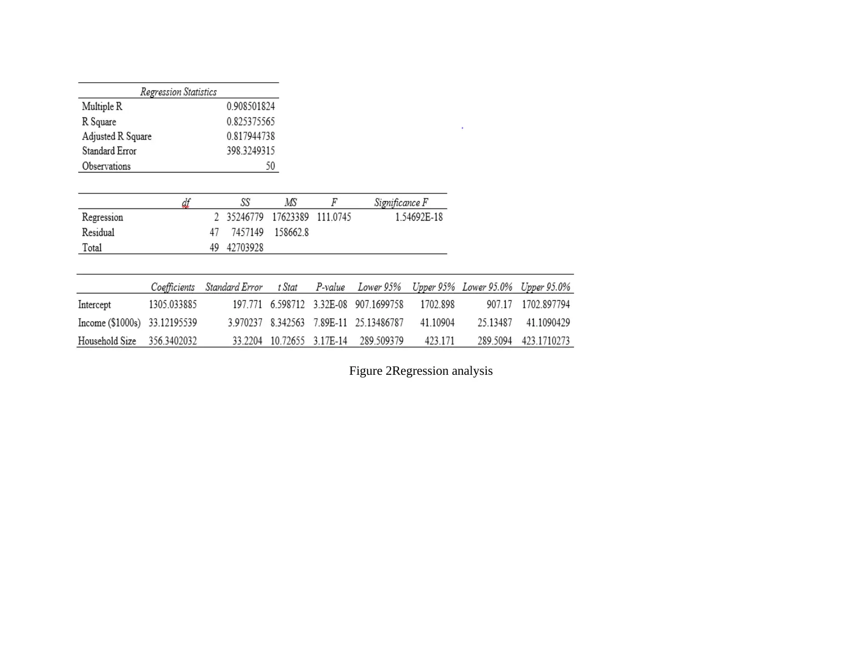
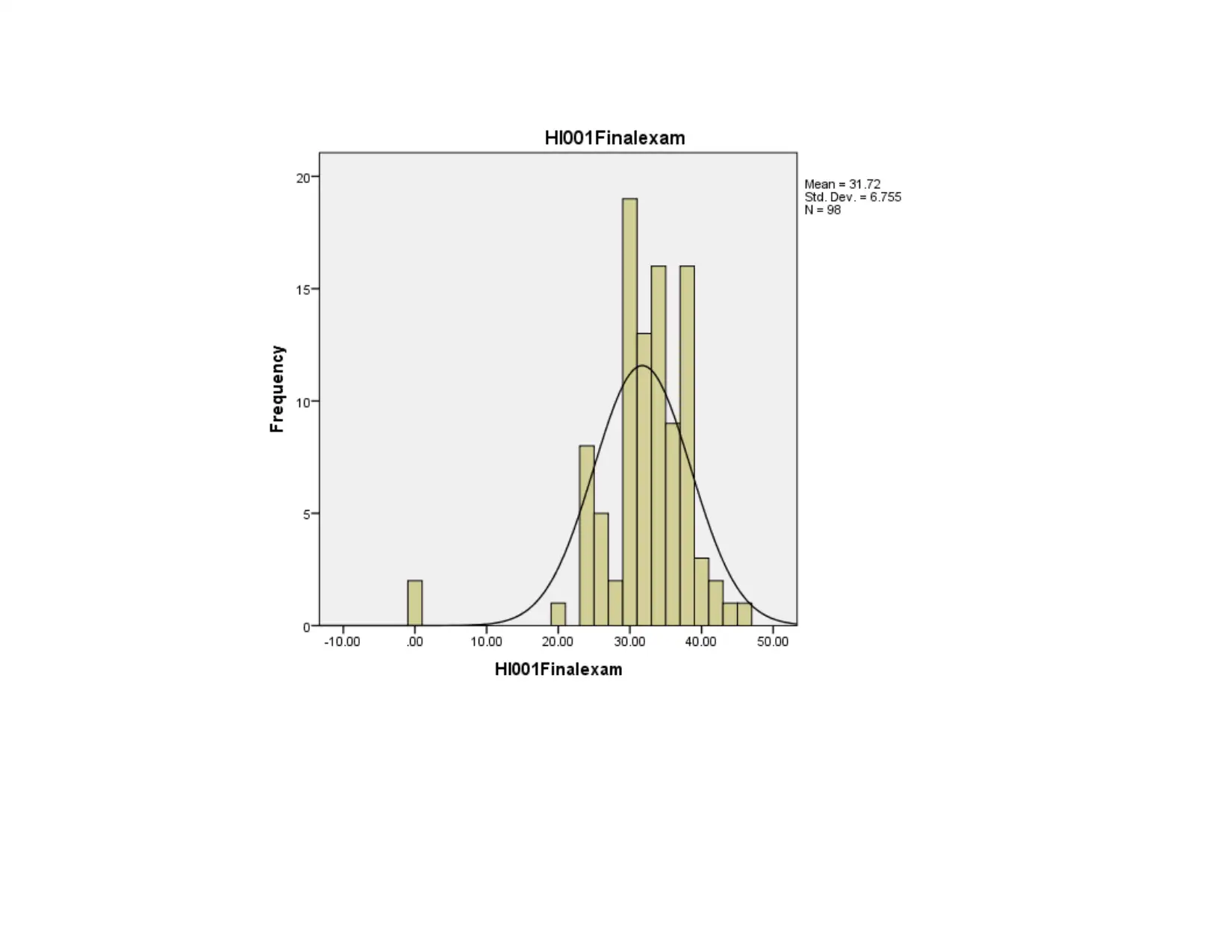
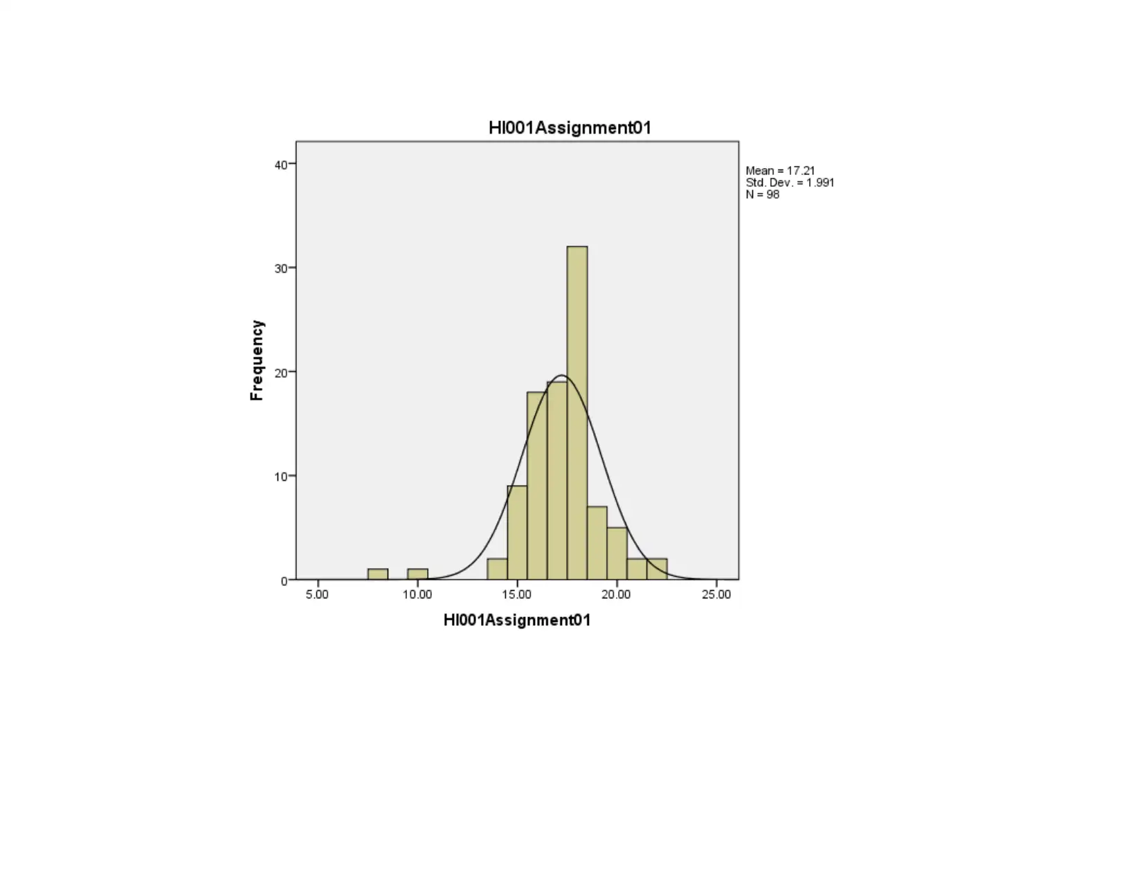
This report presents a statistical analysis of credit card data, employing descriptive statistics and regression analysis to explore relationships between variables such as income, household size, and credit card charges. The analysis includes regression equations, predicted credit card charges, and model modifications. Task 2 focuses on exam and assignment scores, utilizing histograms, descriptive statistics, and correlation analysis to identify relationships between different assessments. Task 3 delves into depression levels across different cities, employing descriptive statistics and ANOVA to assess the impact of health status on depression. The report concludes with key findings and implications derived from the statistical analyses.

STATS

TABLE OF CONTENTS
INTRODUCTION.......................................................................................................................................................................................3
TASK 1........................................................................................................................................................................................................3
1 Descriptive statistics.............................................................................................................................................................................3
2 Regression analysis...............................................................................................................................................................................4
3 Equation of regression..........................................................................................................................................................................8
4 Predicted credit card charge when family size is three.........................................................................................................................8
5 Modification of model..........................................................................................................................................................................9
TASK 2......................................................................................................................................................................................................10
Activity 01.............................................................................................................................................................................................10
Activity 02.............................................................................................................................................................................................10
Activity 03.............................................................................................................................................................................................22
TASK 3......................................................................................................................................................................................................25
1 Descriptive statistics...........................................................................................................................................................................25
2 ANNOVA...........................................................................................................................................................................................25
3 Appropriateness of treatment..............................................................................................................................................................27
CONCLUSION..........................................................................................................................................................................................27

INTRODUCTION
In the current time period credit card business is running by the number of firms. In the current report data set related to credit
card is analyzed and in this regard descriptive statistical tool are used to analyze the data along with regression analysis tools. In
middle part of the report, correlation tool is applied to explore relationship among the variables. Apart from this, ANOVA tools is
used to identify whether there is relationship between geographic location and depression level. In this way, entire research is carried
out.
TASK 1
1 Descriptive statistics
Figure 1Descriptive statistics details
Interpretation

In case of variable income it is observed that on average basis people are earning $43000 followed by standard deviation which is
14.55. On other hand, in case of variable household on average basis size of the entire family is 3.42 which means that on average
basis there are 3 to 4 members in each family from whom data is gathered. Standard deviation is 1.73 which means that family size is
approx. same over time period and it does not change at rapid pace. Mean value of amount charged is 3963.86 which means that there
are large number of respondents which are making annual charge of mentioned value in respect to credit card. Results are clearly
reflecting that the difference between minimum and maximum amount charged is high if same is compared with relevant studied
variables which are given in the table. This is reflecting that people become more habitual of using credit card to meet their needs.
Even people are making overuse of credit card if we compare and take in to account their income level.
2 Regression analysis
H0: There is no significant mean difference between income level, household size and amount charged.
H1: There is significant mean difference between income level, household size and amount charged.

Figure 2Regression analysis

Figure 3Income residual chart
Figure 4Household size chart

Figure 5Income line fit plot
Figure 6Household size line fit plot
Interpretation

There is high degree of correlation among the variables income level, household and amount charged. This is proved from the
fact the correlation value is 0.90 which is very high and is near to 1. Results are also indicating that big percentage change comes in
the amount spend with slight change that happened in the values of the variables namely income level and household. As per facts
82% variation comes in the amount spend with variation in the mentioned variables. Adjusted R square is 0.81 which strongly
indicating that 81% variation comes in the amount charged when any new variable will be added in the data set. Level of significance
is 1.54>0.05 and this is clear that in terms of impact both independent variables does not have significant impact on the dependent
variable. Results are reflecting that in case income of individual changed then amount charged may be impacted by 33 points. In same
way if household size altered then amount charged may change by 356 points.
3 Equation of regression
Regression equation for income level and household are prepared above. It can be observed that value of intercept is 1305 and same of
beta is different in case of income level and household which are 33.12 and 356. X is the dependent variable. When value of
dependent variable is placed in the above mentioned model value for dependent variable is computed. It can be said that regression
analysis is the one of the most important tool that is used to make prediction for dependent variable.
4 Predicted credit card charge when family size is three
Household size= a+ bx
= 1305+356*3=2373
Results are clearly indicating that on mean basis average charge may be of value $2373 in case people income is $40000.

5 Modification of model
Model can be modified by adding new variable namely household saving rate and by using relationship that exist between the
saving rate and credit card charge can be identified.

TASK 2
Activity 01
Data are arranged in variable view in excel sheet.
Activity 02
(a)Drawing histogram

(b)Descriptive statistics
Interpretation
On analysis of variables it can be observed that mean value and standard deviation of HI003 final exam is 25.99(8.27). Value
of both statistical tools in case of HI002 final exam is 17.82(3.44) followed by 33.296(4.99) for HI001 final exam. It can be said that
students are scoring high number of marks in case of HI001 final exam relative to other one. However, scoring is deviating at fast rate
in case of HI003 final exam in comparison to other one. Minmium scoring is done by the students in HI003 final exam and this
reflects that performnace of students is very low in case of HI003 final exam.

Activity 03

Interpretation
 HI001 final exam: Mentioned variable have positive and negative correlation with the other variables. It can be observed that
mentioned variable is positively related with HI001 and HI003 2 assignments. In both cases value of level of significance
where 0.01 and 0.03<0.05. There is negative relation of the variable with HI002 1st test and same of the HI003. Thus, it can be
said that HI001 have both positive and negative correlation with variables.
 H1001 assignment 01: Results are clearly indicating that HI001 assignments and final exam that is related to HI003. It can be
seen from the above table that in case of HI002 final exam and first assignment of same there is negative correlation -0.15 and
-0.97. Thus, variable have both positive and negative relationship with other variables.
 HI001 assignment 02: Related variable have low correlation with HI003 final exam as value of statistical tool is 0.277as well
as same for HI003 assignment 1 is 0.049. Other than this in case of all other variables negative correlation is observed in
respect to HI001 assignment 02.
 HI002 final exam: HI002 final exam is associated with its first and second assignment values positively. As it can be observed
that value of level of significance is 0.177(0.081>0.05 and 0.363(0.00>0.05), HI003 final exam 0.116(0.257>0.05). Mentioned
variable have less of medium relationship with HI003 final exam. Thus, it can be said that there is interconnection among
variables.
 HI002 assignment 01: Results are clearly revealing the relationship that HI002 assignment 01 have with the second
assignment of HI002 and final exam of HI003. Correlation value is 0.549(0.00>0.05) and 0.016(0.880>0.05) for both
variables. There is negative association of HI002 assignment 01 first assignment of HI003. This is proved from the negative
value of correlation -232(0.02<0.05) and second assignment of HI003 -0.74(0.470).
 HI002 assignment 02: It can be seen from the table that final exam of HI003 is positively related to second assignment of
HI002. There is negative correlation of variable with first assignment of HI003 -.192(0.05=0.05). Same trend is observed in
case of third assignment of HI003.

 HI003 final exam: Results are reflecting that assignment one of HI003 and second assignment of HI003 are positively related
with correlation value of 0.197(0.05=0.05). Same trend is observed in case of second assignment of HI003.
 HI003 assignment 01: Assignment 1 and assignment 2 values are related to each other as reflected by 0.520 (0.00<0.05). It
can be said that marks of first assignment if reduced then same thing will be observed in case of other assignment.
TASK 3
1 Descriptive statistics
Table 1Descriptive statistics tools
Florida New
York
North
Carolina Florida New
York
North
Carolina
Mean 5.55 8 7.05 14.5 15.25 13.95
STDEV 6 8 7.5 14.5 14.5 14
MAX 9 13 12 21 24 19
MIN 2 4 3 9 9 8
Interpretation
Mean value of depression is high in case of North Carolina in case respondents are good in health. Depression level is not
deviating at higher rate in case of all these three cities as standard deviation value is 6, 8 and 7.5. In case respondents taken are
suffered from any disease it is observed depression level become double in terms of mean value and standard deviation. It can be said
that disease heavily put impact on depression level.
2 ANNOVA
H0: There is no significant mean difference in depression level across studied cities when people are healthy.
HI: There is significant mean difference in depression level across studied cities when people are healthy.

Interpretation
P value is 0.00<0.05 which means that there is significant mean difference between mean value of depression across cities. It
can be said that city wise depression level very.
H0: There is no significant mean difference in depression level across studied cities when people are not healthy.
HI: There is significant mean difference in depression level across studied cities when people are not healthy.

Interpretation
Value of level of significance is 0.49>0.05 which reflects that there is no significant difference in mean value of depression
across different studied cities. It can be said that depression level remain same if one is suffered from specific disease.
3 Appropriateness of treatment
Those who are suffered from depression can do yoga and meditation to control depression level to great extent. By doing so
they can control depression and can live healthy life
CONCLUSION
It is deduced that amount charged is not affected by household size and income level significantly. Means that change in these
variables does not bring big change in dependent variable. It is also concluded that marks of one test does not heavily affects marks
that can be obtained on other tests as reflected by regression analysis tools. It is also concluded that across the cities depression level is

different when patients are healthy. However, in case they are suffered from any disease then in that case depression level does not
vary among cities.