Credit Scoring Model Development and Analysis - [Course Name]

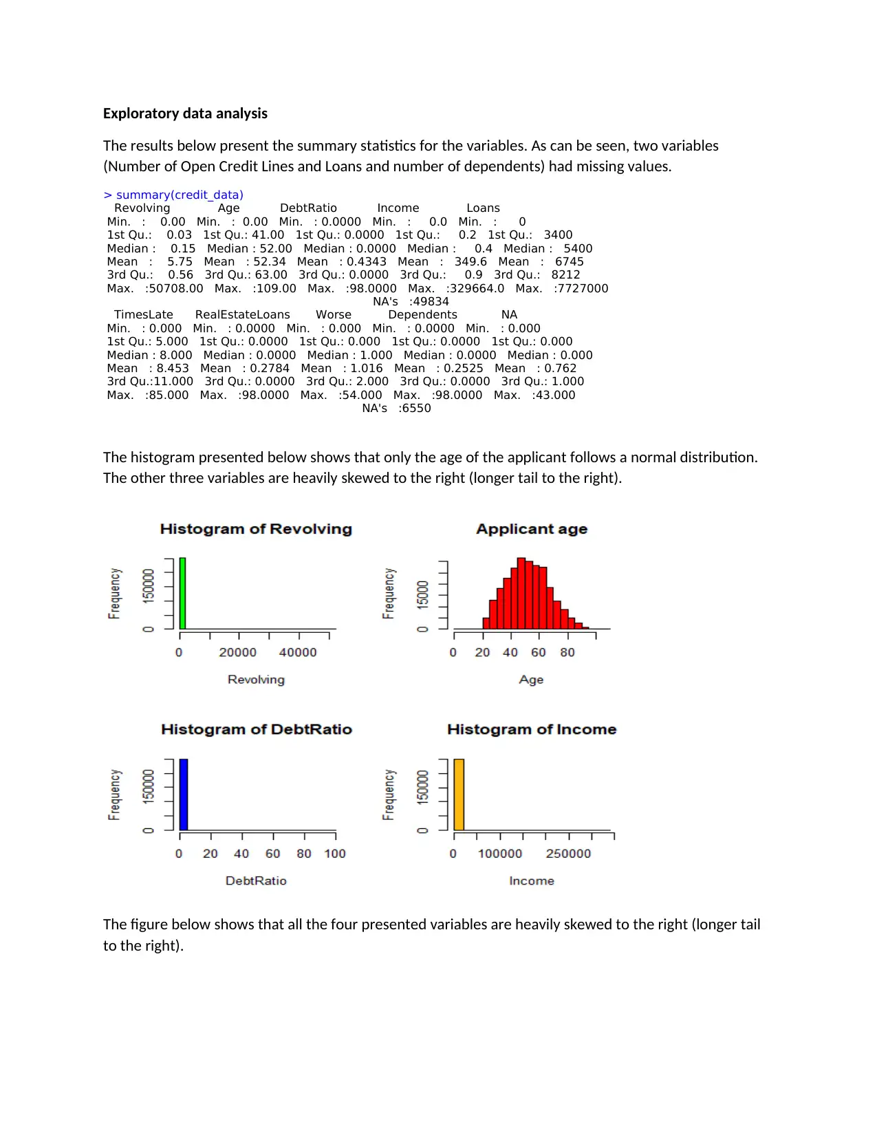
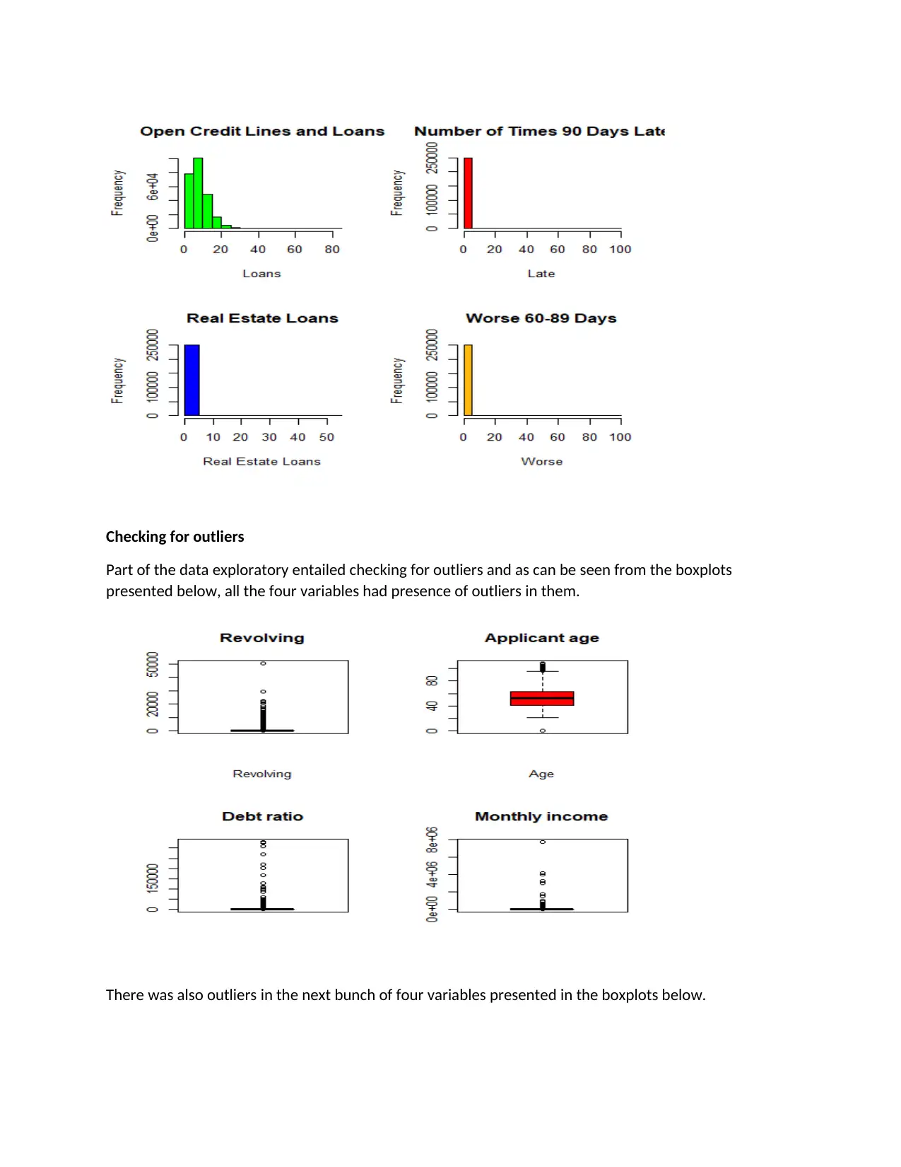
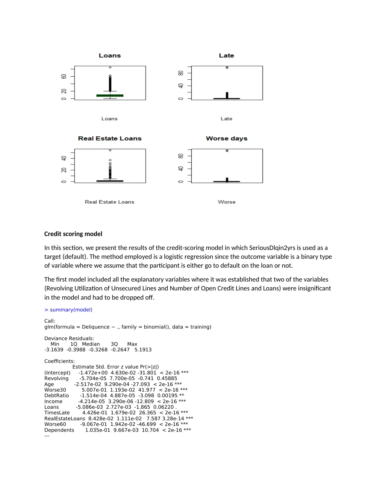
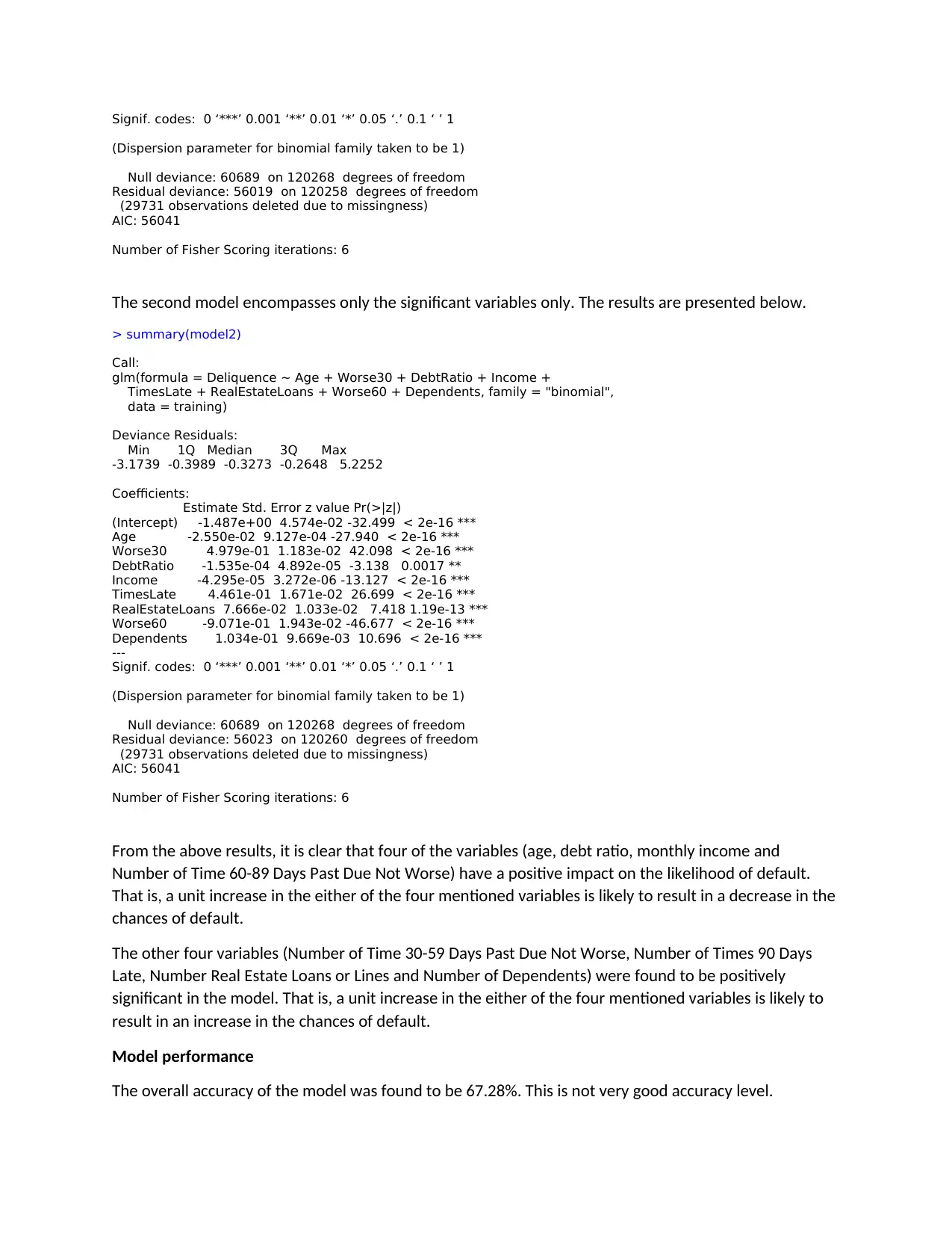
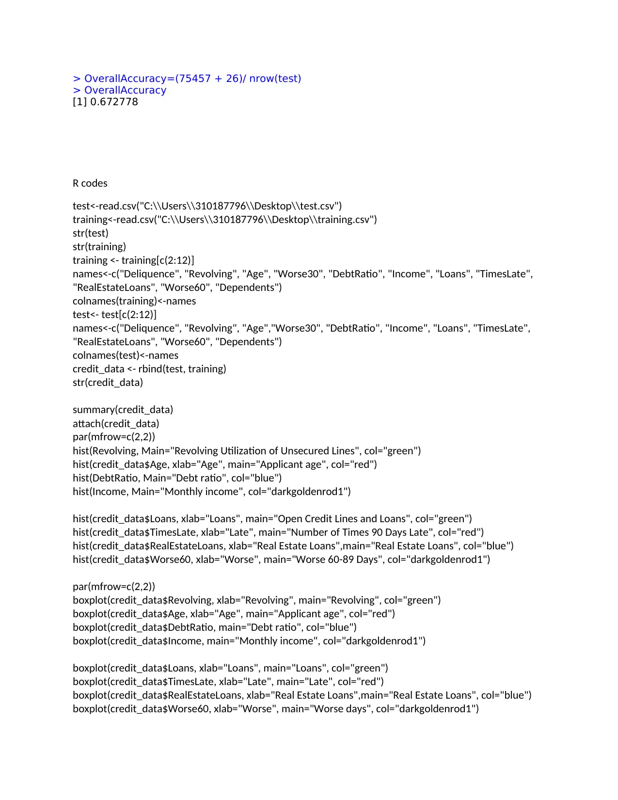
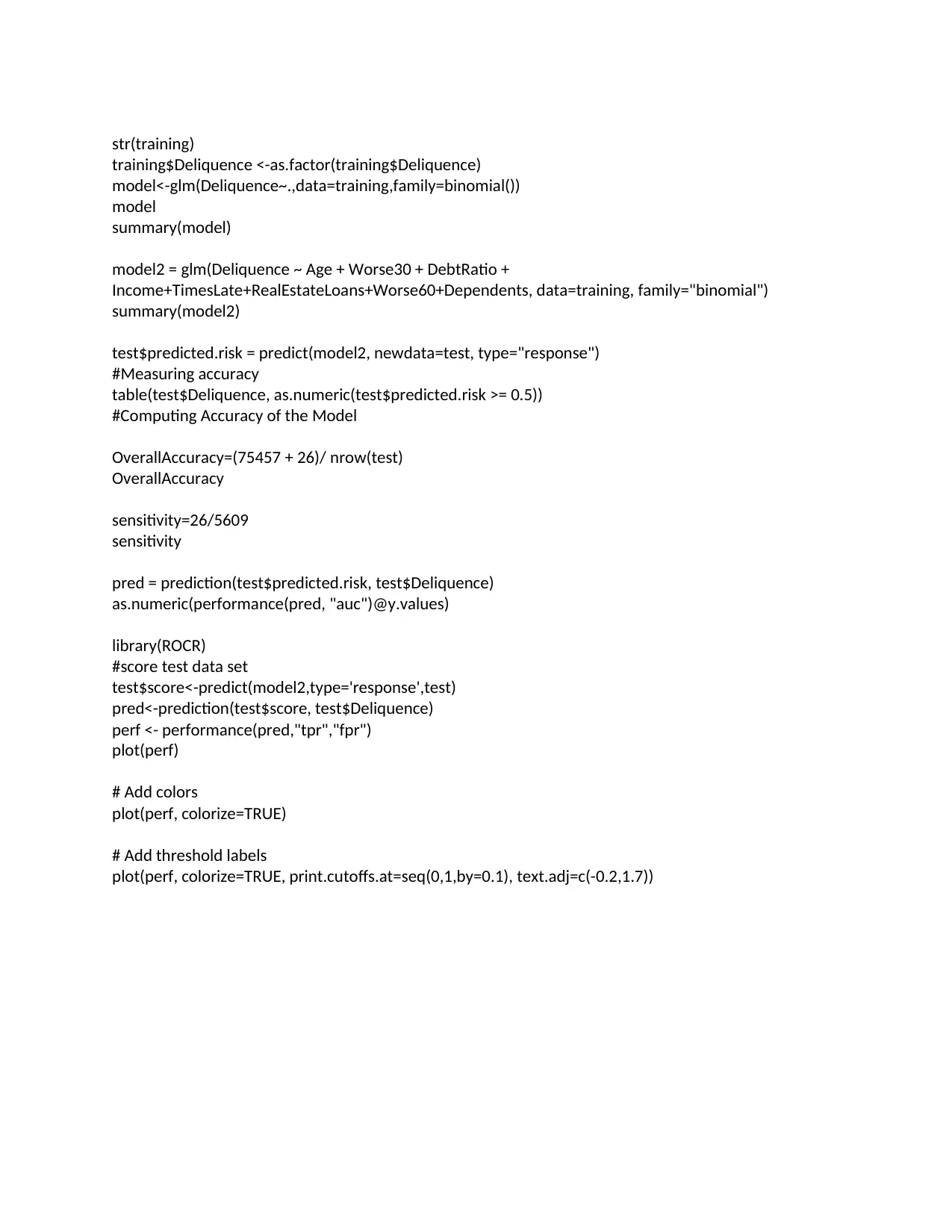
This assignment presents a credit scoring model developed using a dataset of 150,000 borrowers. The analysis begins with exploratory data analysis (EDA) to understand the distribution of variables, identify missing values, and detect outliers. The EDA reveals that some variables are heavily skewed and contain outliers. A logistic regression model is then built to predict the probability of default (SeriousDlqin2yrs). The initial model includes all explanatory variables, but insignificant variables are dropped in the second model. The results show that certain variables (age, debt ratio, monthly income, and past due) have a positive impact on the likelihood of default, while others have a negative impact. The model's overall accuracy is 67.28%. The R code used for data loading, preprocessing, model building, and evaluation is also provided. The assignment demonstrates the application of data mining techniques in credit risk assessment.

Credit Scoring
Student Name:
Instructor Name:
Course Number:
29th March 2020

Exploratory data analysis
The results below present the summary statistics for the variables. As can be seen, two variables
(Number of Open Credit Lines and Loans and number of dependents) had missing values.
> summary(credit_data)
Revolving Age DebtRatio Income Loans
Min. : 0.00 Min. : 0.00 Min. : 0.0000 Min. : 0.0 Min. : 0
1st Qu.: 0.03 1st Qu.: 41.00 1st Qu.: 0.0000 1st Qu.: 0.2 1st Qu.: 3400
Median : 0.15 Median : 52.00 Median : 0.0000 Median : 0.4 Median : 5400
Mean : 5.75 Mean : 52.34 Mean : 0.4343 Mean : 349.6 Mean : 6745
3rd Qu.: 0.56 3rd Qu.: 63.00 3rd Qu.: 0.0000 3rd Qu.: 0.9 3rd Qu.: 8212
Max. :50708.00 Max. :109.00 Max. :98.0000 Max. :329664.0 Max. :7727000
NA's :49834
TimesLate RealEstateLoans Worse Dependents NA
Min. : 0.000 Min. : 0.0000 Min. : 0.000 Min. : 0.0000 Min. : 0.000
1st Qu.: 5.000 1st Qu.: 0.0000 1st Qu.: 0.000 1st Qu.: 0.0000 1st Qu.: 0.000
Median : 8.000 Median : 0.0000 Median : 1.000 Median : 0.0000 Median : 0.000
Mean : 8.453 Mean : 0.2784 Mean : 1.016 Mean : 0.2525 Mean : 0.762
3rd Qu.:11.000 3rd Qu.: 0.0000 3rd Qu.: 2.000 3rd Qu.: 0.0000 3rd Qu.: 1.000
Max. :85.000 Max. :98.0000 Max. :54.000 Max. :98.0000 Max. :43.000
NA's :6550
The histogram presented below shows that only the age of the applicant follows a normal distribution.
The other three variables are heavily skewed to the right (longer tail to the right).
The figure below shows that all the four presented variables are heavily skewed to the right (longer tail
to the right).

Checking for outliers
Part of the data exploratory entailed checking for outliers and as can be seen from the boxplots
presented below, all the four variables had presence of outliers in them.
There was also outliers in the next bunch of four variables presented in the boxplots below.

Credit scoring model
In this section, we present the results of the credit-scoring model in which SeriousDlqin2yrs is used as a
target (default). The method employed is a logistic regression since the outcome variable is a binary type
of variable where we assume that the participant is either go to default on the loan or not.
The first model included all the explanatory variables where it was established that two of the variables
(Revolving Utilization of Unsecured Lines and Number of Open Credit Lines and Loans) were insignificant
in the model and had to be dropped off.
> summary(model)
Call:
glm(formula = Deliquence ~ ., family = binomial(), data = training)
Deviance Residuals:
Min 1Q Median 3Q Max
-3.1639 -0.3988 -0.3268 -0.2647 5.1913
Coefficients:
Estimate Std. Error z value Pr(>|z|)
(Intercept) -1.472e+00 4.630e-02 -31.801 < 2e-16 ***
Revolving -5.704e-05 7.700e-05 -0.741 0.45885
Age -2.517e-02 9.290e-04 -27.093 < 2e-16 ***
Worse30 5.007e-01 1.193e-02 41.977 < 2e-16 ***
DebtRatio -1.514e-04 4.887e-05 -3.098 0.00195 **
Income -4.214e-05 3.290e-06 -12.809 < 2e-16 ***
Loans -5.086e-03 2.727e-03 -1.865 0.06220 .
TimesLate 4.426e-01 1.679e-02 26.365 < 2e-16 ***
RealEstateLoans 8.428e-02 1.111e-02 7.587 3.28e-14 ***
Worse60 -9.067e-01 1.942e-02 -46.699 < 2e-16 ***
Dependents 1.035e-01 9.667e-03 10.704 < 2e-16 ***
---

Signif. codes: 0 ‘***’ 0.001 ‘**’ 0.01 ‘*’ 0.05 ‘.’ 0.1 ‘ ’ 1
(Dispersion parameter for binomial family taken to be 1)
Null deviance: 60689 on 120268 degrees of freedom
Residual deviance: 56019 on 120258 degrees of freedom
(29731 observations deleted due to missingness)
AIC: 56041
Number of Fisher Scoring iterations: 6
The second model encompasses only the significant variables only. The results are presented below.
> summary(model2)
Call:
glm(formula = Deliquence ~ Age + Worse30 + DebtRatio + Income +
TimesLate + RealEstateLoans + Worse60 + Dependents, family = "binomial",
data = training)
Deviance Residuals:
Min 1Q Median 3Q Max
-3.1739 -0.3989 -0.3273 -0.2648 5.2252
Coefficients:
Estimate Std. Error z value Pr(>|z|)
(Intercept) -1.487e+00 4.574e-02 -32.499 < 2e-16 ***
Age -2.550e-02 9.127e-04 -27.940 < 2e-16 ***
Worse30 4.979e-01 1.183e-02 42.098 < 2e-16 ***
DebtRatio -1.535e-04 4.892e-05 -3.138 0.0017 **
Income -4.295e-05 3.272e-06 -13.127 < 2e-16 ***
TimesLate 4.461e-01 1.671e-02 26.699 < 2e-16 ***
RealEstateLoans 7.666e-02 1.033e-02 7.418 1.19e-13 ***
Worse60 -9.071e-01 1.943e-02 -46.677 < 2e-16 ***
Dependents 1.034e-01 9.669e-03 10.696 < 2e-16 ***
---
Signif. codes: 0 ‘***’ 0.001 ‘**’ 0.01 ‘*’ 0.05 ‘.’ 0.1 ‘ ’ 1
(Dispersion parameter for binomial family taken to be 1)
Null deviance: 60689 on 120268 degrees of freedom
Residual deviance: 56023 on 120260 degrees of freedom
(29731 observations deleted due to missingness)
AIC: 56041
Number of Fisher Scoring iterations: 6
From the above results, it is clear that four of the variables (age, debt ratio, monthly income and
Number of Time 60-89 Days Past Due Not Worse) have a positive impact on the likelihood of default.
That is, a unit increase in the either of the four mentioned variables is likely to result in a decrease in the
chances of default.
The other four variables (Number of Time 30-59 Days Past Due Not Worse, Number of Times 90 Days
Late, Number Real Estate Loans or Lines and Number of Dependents) were found to be positively
significant in the model. That is, a unit increase in the either of the four mentioned variables is likely to
result in an increase in the chances of default.
Model performance
The overall accuracy of the model was found to be 67.28%. This is not very good accuracy level.

> OverallAccuracy=(75457 + 26)/ nrow(test)
> OverallAccuracy
[1] 0.672778
R codes
test<-read.csv("C:\\Users\\310187796\\Desktop\\test.csv")
training<-read.csv("C:\\Users\\310187796\\Desktop\\training.csv")
str(test)
str(training)
training <- training[c(2:12)]
names<-c("Deliquence", "Revolving", "Age", "Worse30", "DebtRatio", "Income", "Loans", "TimesLate",
"RealEstateLoans", "Worse60", "Dependents")
colnames(training)<-names
test<- test[c(2:12)]
names<-c("Deliquence", "Revolving", "Age","Worse30", "DebtRatio", "Income", "Loans", "TimesLate",
"RealEstateLoans", "Worse60", "Dependents")
colnames(test)<-names
credit_data <- rbind(test, training)
str(credit_data)
summary(credit_data)
attach(credit_data)
par(mfrow=c(2,2))
hist(Revolving, Main="Revolving Utilization of Unsecured Lines", col="green")
hist(credit_data$Age, xlab="Age", main="Applicant age", col="red")
hist(DebtRatio, Main="Debt ratio", col="blue")
hist(Income, Main="Monthly income", col="darkgoldenrod1")
hist(credit_data$Loans, xlab="Loans", main="Open Credit Lines and Loans", col="green")
hist(credit_data$TimesLate, xlab="Late", main="Number of Times 90 Days Late", col="red")
hist(credit_data$RealEstateLoans, xlab="Real Estate Loans",main="Real Estate Loans", col="blue")
hist(credit_data$Worse60, xlab="Worse", main="Worse 60-89 Days", col="darkgoldenrod1")
par(mfrow=c(2,2))
boxplot(credit_data$Revolving, xlab="Revolving", main="Revolving", col="green")
boxplot(credit_data$Age, xlab="Age", main="Applicant age", col="red")
boxplot(credit_data$DebtRatio, main="Debt ratio", col="blue")
boxplot(credit_data$Income, main="Monthly income", col="darkgoldenrod1")
boxplot(credit_data$Loans, xlab="Loans", main="Loans", col="green")
boxplot(credit_data$TimesLate, xlab="Late", main="Late", col="red")
boxplot(credit_data$RealEstateLoans, xlab="Real Estate Loans",main="Real Estate Loans", col="blue")
boxplot(credit_data$Worse60, xlab="Worse", main="Worse days", col="darkgoldenrod1")

str(training)
training$Deliquence <-as.factor(training$Deliquence)
model<-glm(Deliquence~.,data=training,family=binomial())
model
summary(model)
model2 = glm(Deliquence ~ Age + Worse30 + DebtRatio +
Income+TimesLate+RealEstateLoans+Worse60+Dependents, data=training, family="binomial")
summary(model2)
test$predicted.risk = predict(model2, newdata=test, type="response")
#Measuring accuracy
table(test$Deliquence, as.numeric(test$predicted.risk >= 0.5))
#Computing Accuracy of the Model
OverallAccuracy=(75457 + 26)/ nrow(test)
OverallAccuracy
sensitivity=26/5609
sensitivity
pred = prediction(test$predicted.risk, test$Deliquence)
as.numeric(performance(pred, "auc")@y.values)
library(ROCR)
#score test data set
test$score<-predict(model2,type='response',test)
pred<-prediction(test$score, test$Deliquence)
perf <- performance(pred,"tpr","fpr")
plot(perf)
# Add colors
plot(perf, colorize=TRUE)
# Add threshold labels
plot(perf, colorize=TRUE, print.cutoffs.at=seq(0,1,by=0.1), text.adj=c(-0.2,1.7))