Statistical Analysis of Crime Rates and Related Factors

This report presents a statistical analysis of crime rates, exploring various factors and their significance. Section A examines whether southern states have higher crime rates, the relationship between crime rates and police expenditure, changes in crime rates over 10 years, and youth unemploymen...Read More

Applied Research Methods

Table of Contents
Section A.........................................................................................................................................3
Section B..........................................................................................................................................5

Section A
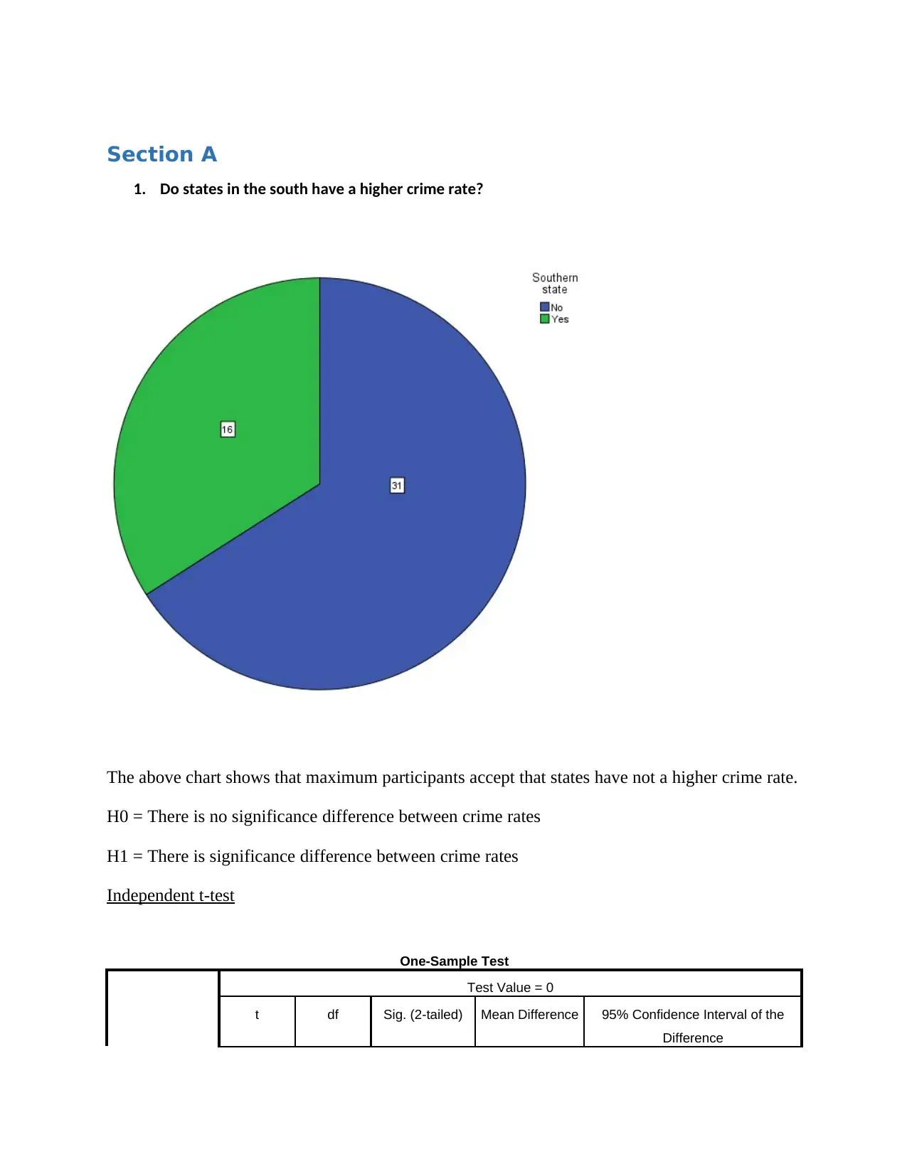
1. Do states in the south have a higher crime rate?
The above chart shows that maximum participants accept that states have not a higher crime rate.
H0 = There is no significance difference between crime rates
H1 = There is significance difference between crime rates
Independent t-test
One-Sample Test
Test Value = 0
t df Sig. (2-tailed) Mean Difference 95% Confidence Interval of the
Difference

Lower Upper
Southern state 4.873 46 .000 .340 .20 .48
The result indicates the value of t is 4.873, this indicates that there is no significance difference
between crime rate and Southern region.
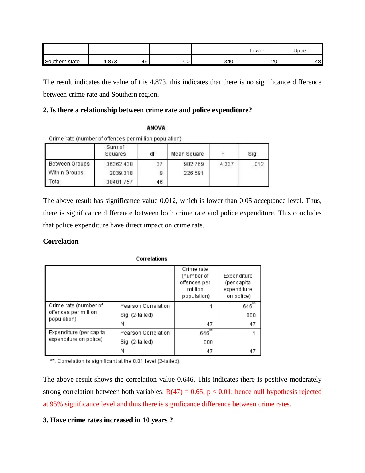
2. Is there a relationship between crime rate and police expenditure?
The above result has significance value 0.012, which is lower than 0.05 acceptance level. Thus,
there is significance difference between both crime rate and police expenditure. This concludes
that police expenditure have direct impact on crime rate.
Correlation
The above result shows the correlation value 0.646. This indicates there is positive moderately
strong correlation between both variables. R(47) = 0.65, p < 0.01; hence null hypothesis rejected
at 95% significance level and thus there is significance difference between crime rates.
3. Have crime rates increased in 10 years ?

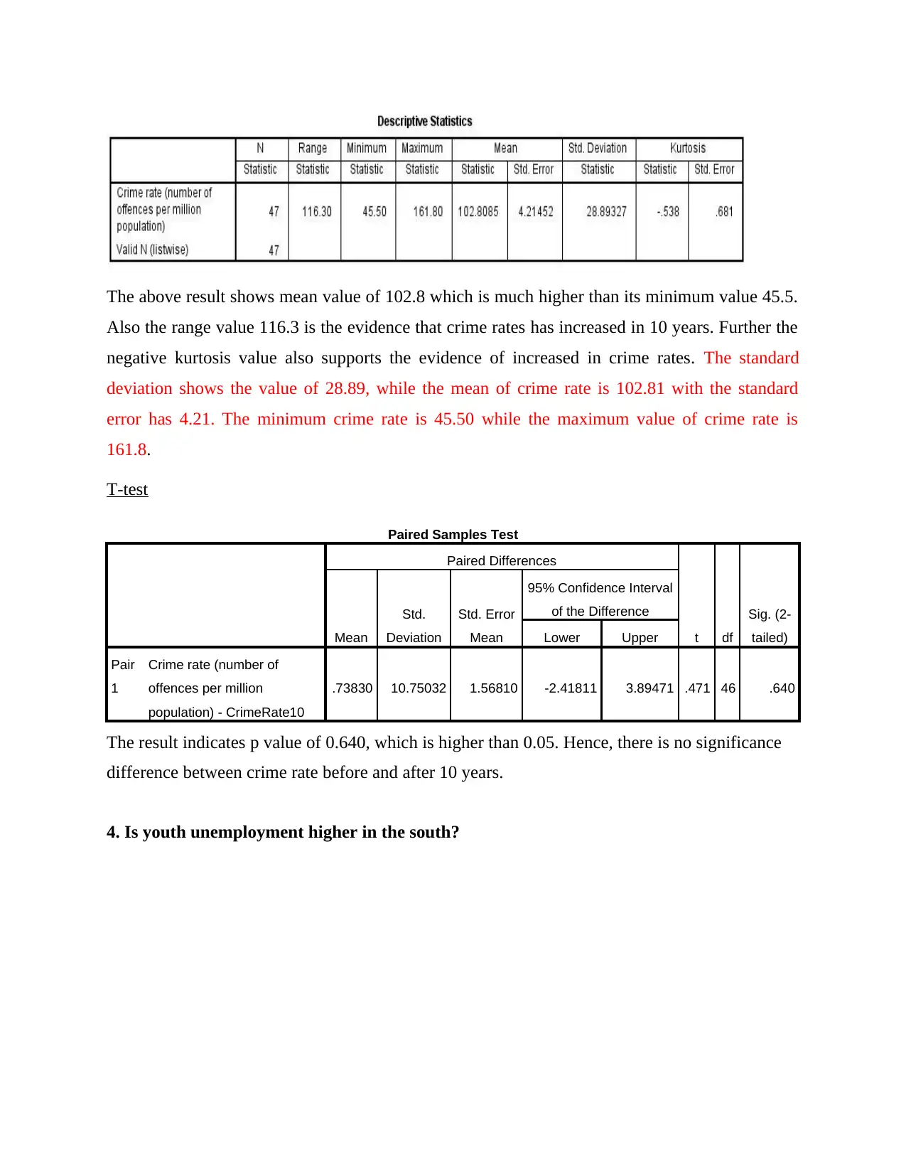
The above result shows mean value of 102.8 which is much higher than its minimum value 45.5.
Also the range value 116.3 is the evidence that crime rates has increased in 10 years. Further the
negative kurtosis value also supports the evidence of increased in crime rates. The standard
deviation shows the value of 28.89, while the mean of crime rate is 102.81 with the standard
error has 4.21. The minimum crime rate is 45.50 while the maximum value of crime rate is
161.8.
T-test
Paired Samples Test
Paired Differences
t df
Sig. (2-
tailed)Mean
Std.
Deviation
Std. Error
Mean
95% Confidence Interval
of the Difference
Lower Upper
Pair
1
Crime rate (number of
offences per million
population) - CrimeRate10
.73830 10.75032 1.56810 -2.41811 3.89471 .471 46 .640
The result indicates p value of 0.640, which is higher than 0.05. Hence, there is no significance
difference between crime rate before and after 10 years.
4. Is youth unemployment higher in the south?

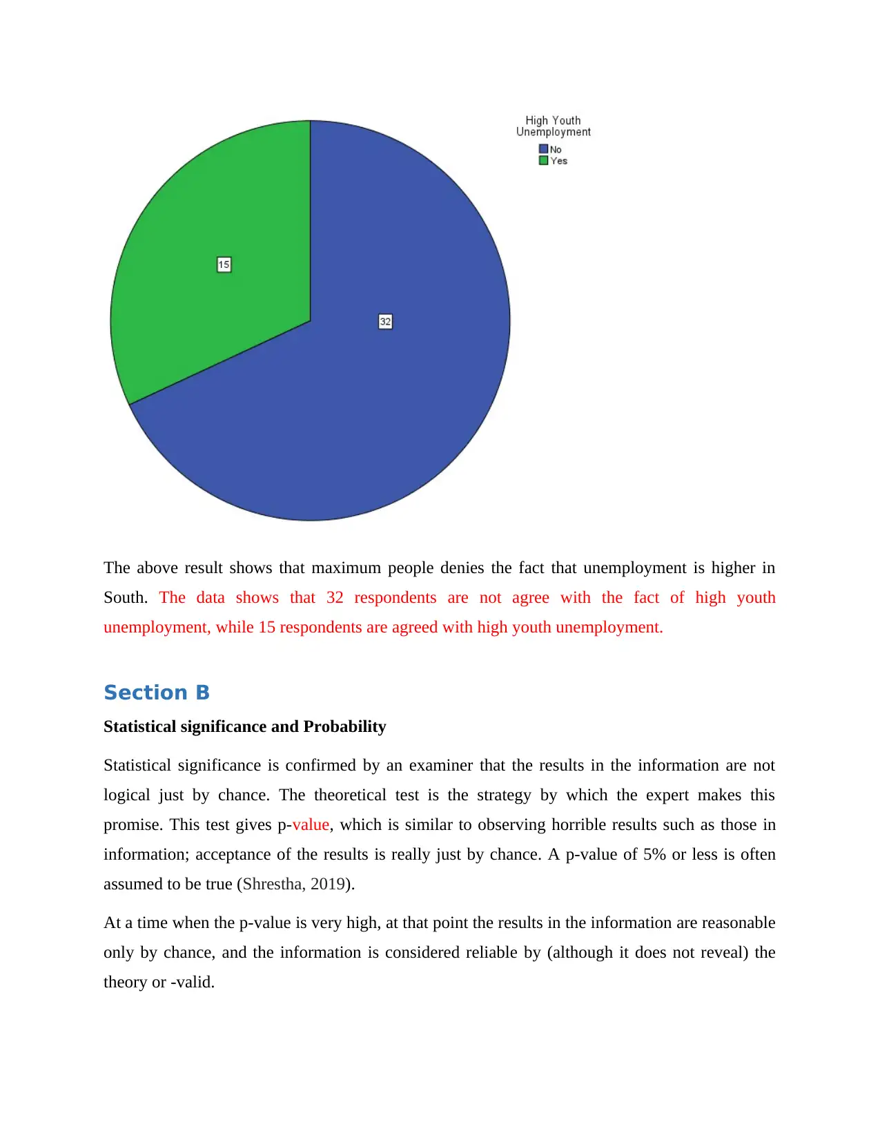
The above result shows that maximum people denies the fact that unemployment is higher in
South. The data shows that 32 respondents are not agree with the fact of high youth
unemployment, while 15 respondents are agreed with high youth unemployment.
Section B
Statistical significance and Probability
Statistical significance is confirmed by an examiner that the results in the information are not
logical just by chance. The theoretical test is the strategy by which the expert makes this
promise. This test gives p-value, which is similar to observing horrible results such as those in
information; acceptance of the results is really just by chance. A p-value of 5% or less is often
assumed to be true (Shrestha, 2019).
At a time when the p-value is very high, at that point the results in the information are reasonable
only by chance, and the information is considered reliable by (although it does not reveal) the
theory or -valid.

A statistically significant p-value is less than 0.05 (typically less than or equal to 0.05). Because
there is a fewer than 5% probability that the null hypothesis is correct, this provides strong
evidence against it (and random outcome). As a result, the null hypothesis is rejected and the
alternative hypothesis is accepted. The null hypothesis can be rejected if the p-value is less than
the significance level (usually p 0.05), but this does not indicate that the alternative hypothesis is
95 percent accurate. The P-value is determined by the truth or falsity of the null hypothesis, but it
has no bearing on the truth or falsity of the alternative hypothesis (Abadie, 2020).
A p-value larger than 0.05 (>0.05) is not statistically significant and indicates that the null
hypothesis is strongly supported. This indicates we're sticking with the null hypothesis and
rejecting the alternative. You can't accept the null hypothesis, and you may either reject it or
embrace it. Enter the precise value of p (e.g., p = 0.031) with two or three decimal places for
reporting p-values. With p 0.001, however, enter a p value smaller than 0.001. When just a few
tables with thresholds were accessible, the practise of reporting p-values in the form p 0.10, p
0.05, p 0.01, and so on was appropriate.
A step-by-step guide to selecting exams and measurable assumptions about test:
As for the choice of reality test, the main study is "what is the main fact test?" sometimes there is
no theory; the researcher only has to "see what it is". For example, in a close relationship there is
no profitability for a test and the size of the test depends on how precise the specialist has to
make a decision. Assuming there is no theory, there is no test of fact. It is important to determine
what profits are proven (i.e., they are trying an alleged relationship) and investigative (the
information is commendable). One test cannot support a complete settlement of profiteering. It is
a reasonable condition to severely limit the amount of profitability that is guaranteed. Although it
is substantial to use factual tests of profitability suggested by the information, P estimates should
be used primarily as rules, and results should be treated as a condition until they are confirmed
by the resulting considerations. A valuable guide is the use of Bonferroni correction, which
basically states that if an attempt is made for autonomous profiteering, a significance level of
0.05 / n should be used. In this way, if there were two autonomous profiteering, a so-called result
would be necessary if P <0.025. Note that since free trials are rare, this is a very traditional
approach, for example one that does not avoid an invalid theory. The specialist should then ask
"Is the information autonomous?" This can be difficult to choose, but reliable management

results on a similar person, or coordinated by people, are not free. In this way, the results from a
pre-hybrid, or from a condensed case-control in which the controls are coordinated to the issues
by age, sex and social class, are not independent (Tenny and Abdelgawad, 2017).
Reality tests expect invalid profits with no relationship or difference between collections. They
then decide whether the information collected falls outside the scope of the expected
characteristics of the invalid profit.
Parametric tests usually have stricter precursors than neutral tests and can produce more basic
results from the information. They need to be guided by information that quickly conforms to
underlying suspicions in reality tests (Ledolter and Kardon, 2020).
The best known types of parametric tests include refraction tests, experimental tests, and bond
tests.
Regression tests
Decay tests are used to determine the locations and connections of logical results. They look for
the influence of at least one constant factor on another variable.
Comparison tests
Research experiments look for differences in meanings. They can be used to test the direct effect
of a factor on the average value of some other brand.
T tests are used when examining methods for two definitive collections (for example, normal
human images). The ANOVA and MANOVA tests are used when examining methods for
multiple assemblies (for example, typical images of young people, adolescents and adults).
Correlation tests
The connection test ensures that two functions are connected without expecting logical
positioning and output results.
They can be used to check if there are two functions to be used (for example) in a series of
automatically linked play tests.
Choosing a nonparametric test

Nonparametric tests don't give much of an impression on the information and are useful when at
least one of the basic truths is not taken into account. However, the stimuli they produce are not
as strong as the parametric tests (Cox, 2020).
Assumptions underlying parametric and non-parametric tests
Non-Parametric
The most important assumptions in nonparametric testing are randomness and freedom. The chi-
square test is one of three types of nonparametric tests that test three types of measurable criteria:
polite, free, and uniform. In nonparametric studies, the Mann-Whitney U test is used to consider
two sets of cases for the variable. The Kruskal-Wallis test is considered an optional one-way
parametric one-way difference analysis (ANOVA) for comparing multiple conclusions on a
single variable. The Wilcoxon Signature Position Test is an optional test for the “paired sample t-
test” to test the average true contrast between two related/inferred random samples.
Parametric
 General: The data has a general (or proportional) distribution.
 Device change: There are similar variations on data in different collections.
 Linearity: Data is directly related
 Freedom: data is autonomous
 Level measurement
Variables have one of four rating levels: Nominal, Ordinal, Break, or Relationship. (Sometimes
the scaling and scoring of the proportions are referred to as continuous or scale.) It is important
for researchers to understand the various ratings because these ratings, along with how rating
questions are expressed, determine whether factual research is appropriate.
The fictitious grade of the evaluation is the basic grade of the evaluation. At this level of
evaluation, the number of variables is used unambiguously to sort the information. You can use
alphanumeric words, letters, and pictures in this class. Assume that information about a person is
in a place with three gender classifications. In this situation, an individual with female sexual
orientation can be called F, and an individual with male gender can be delegated to M and
transgender (name T). This type of grouping is an imaginary level of evaluation (Barot,
Burgsteiner and Kolleritsch, 2020).

The second evaluation grade is the regular grade of the evaluation. An assessment of this degree
reflects a certain relationship between perceptions of variables. It is assumed that the double
stunts scored the most amazing in the class. The main title is given in this situation. At this point,
the other classmates get their second highest score (92 points). She gets the next job. The third
bush will be 81 and the third position. The common grade of the assessment shows the degree
application.
The third form of assessment is the scale of the stress assessment. The grade level gives the order
and scale of the scale, but shows that the distance between each bar on the scale is exactly the
same on the scale from low to high. For example, the relaxation grade level could be a double
stunt neurotic score of 10 to 11; this paragraph corresponds to a stunt score of 40 to 41. A typical
picture of this score is Celsius. The distance is in the range of 940°C to 960°C and equal to the
distance in the range of 1000°C to 1020°C.
The fourth valuation ratio is the stock valuation level. With this degree of assessment, the
perception and presence of that segment can also have a value of zero. A scale of zero makes
these points very different from other types of points, even though their properties are similar to
point-level properties. At the shared assessment level, the scale focal segmentation is the same
distance between them.

References
Shrestha, J., 2019. P-Value: A true test of significance in agricultural research.
Abadie, A., 2020. Statistical nonsignificance in empirical economics. American Economic
Review: Insights, 2(2), pp.193-208.
Tenny, S. and Abdelgawad, I., 2017. Statistical significance.
Ledolter, J. and Kardon, R.H., 2020. Focus on Data: Statistical Significance, Effect Size and the
Accumulation of Evidence Achieved by Combining Study Results Through Meta-
analysis. Investigative ophthalmology & visual science, 61(10), pp.32-32.
Cox, D.R., 2020. Statistical significance. Annual Review of Statistics and its Application, 7, pp.1-
10.
Barot, T., Burgsteiner, H. and Kolleritsch, W., 2020, July. Comparison of discrete
autocorrelation functions with regards to statistical significance. In Computer Science On-line
Conference (pp. 257-266). Springer, Cham.