Crime Rate Analysis: Descriptive Statistics Report - County Data

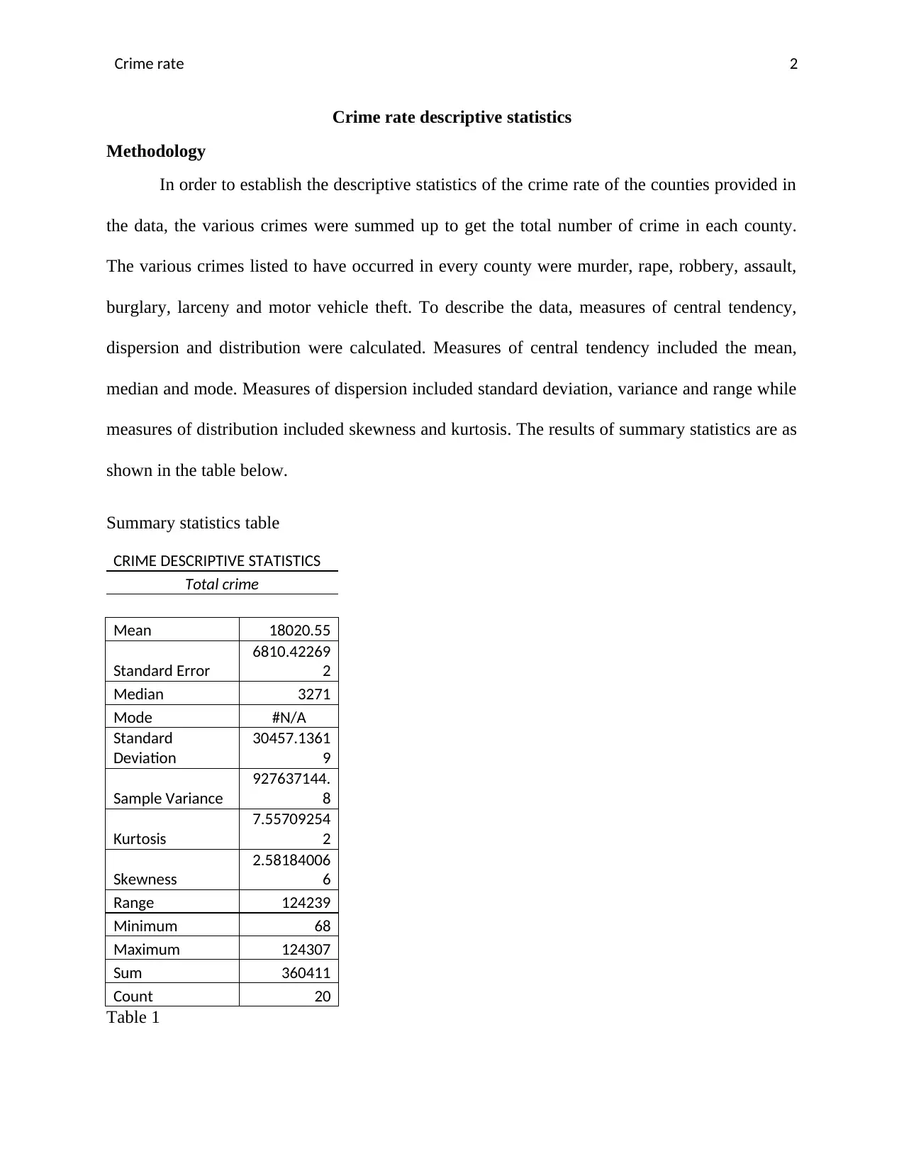
This report presents a crime rate analysis using descriptive statistics. The analysis begins by calculating the total crime for each county, followed by the computation of various statistical measures, including the mean, median, mode, standard deviation, variance, range, skewness, and kurtosis. Th...Read More

Running head: Crime rate 1
Crime rate
Course code:
Student id:
Tutor:

Crime rate 2
Crime rate descriptive statistics
Methodology
In order to establish the descriptive statistics of the crime rate of the counties provided in
the data, the various crimes were summed up to get the total number of crime in each county.
The various crimes listed to have occurred in every county were murder, rape, robbery, assault,
burglary, larceny and motor vehicle theft. To describe the data, measures of central tendency,
dispersion and distribution were calculated. Measures of central tendency included the mean,
median and mode. Measures of dispersion included standard deviation, variance and range while
measures of distribution included skewness and kurtosis. The results of summary statistics are as
shown in the table below.
Summary statistics table
CRIME DESCRIPTIVE STATISTICS
Total crime
Mean 18020.55
Standard Error
6810.42269
2
Median 3271
Mode #N/A
Standard
Deviation
30457.1361
9
Sample Variance
927637144.
8
Kurtosis
7.55709254
2
Skewness
2.58184006
6
Range 124239
Minimum 68
Maximum 124307
Sum 360411
Count 20
Table 1

Crime rate 3
The table above shows the summary statistics of crime rate in the counties. It can be
observed that the average number of crime in the counties is 18020.55 with a standard deviation
of 30,457.14. The median crime was 3271 while the mode could not be established since the data
seemed to have more than two modes. As can be observed the standard error computed was
6810.42. When it comes to distribution, it can be observed that the value of skewness was 2.58.
This means that the crime data was not normally distributed; it was so skewed to the right.
Kurtosis value was also calculated. The data gave a kurtosis value of 7.56 thus showing that the
crime normal curve has a long and sharp apex. In order to rate the counties as low or high crime
counties, it was decided that any county with a crime score of less than 0.00011would be
classified as low crime and any county with crime score from 0.0002 would be classified as high
crime area.