Regression Analysis Report: Purchase Intention and CRM Study

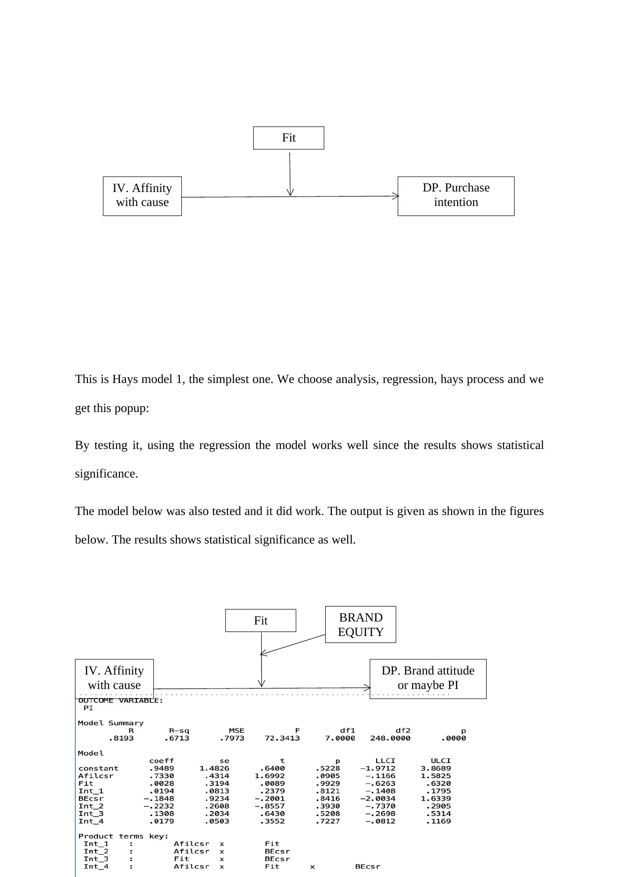
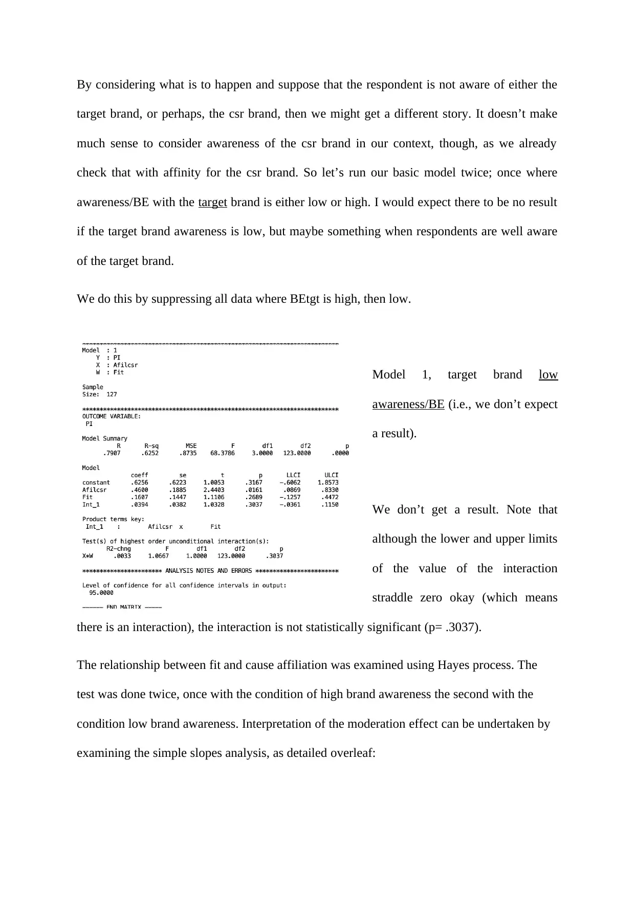
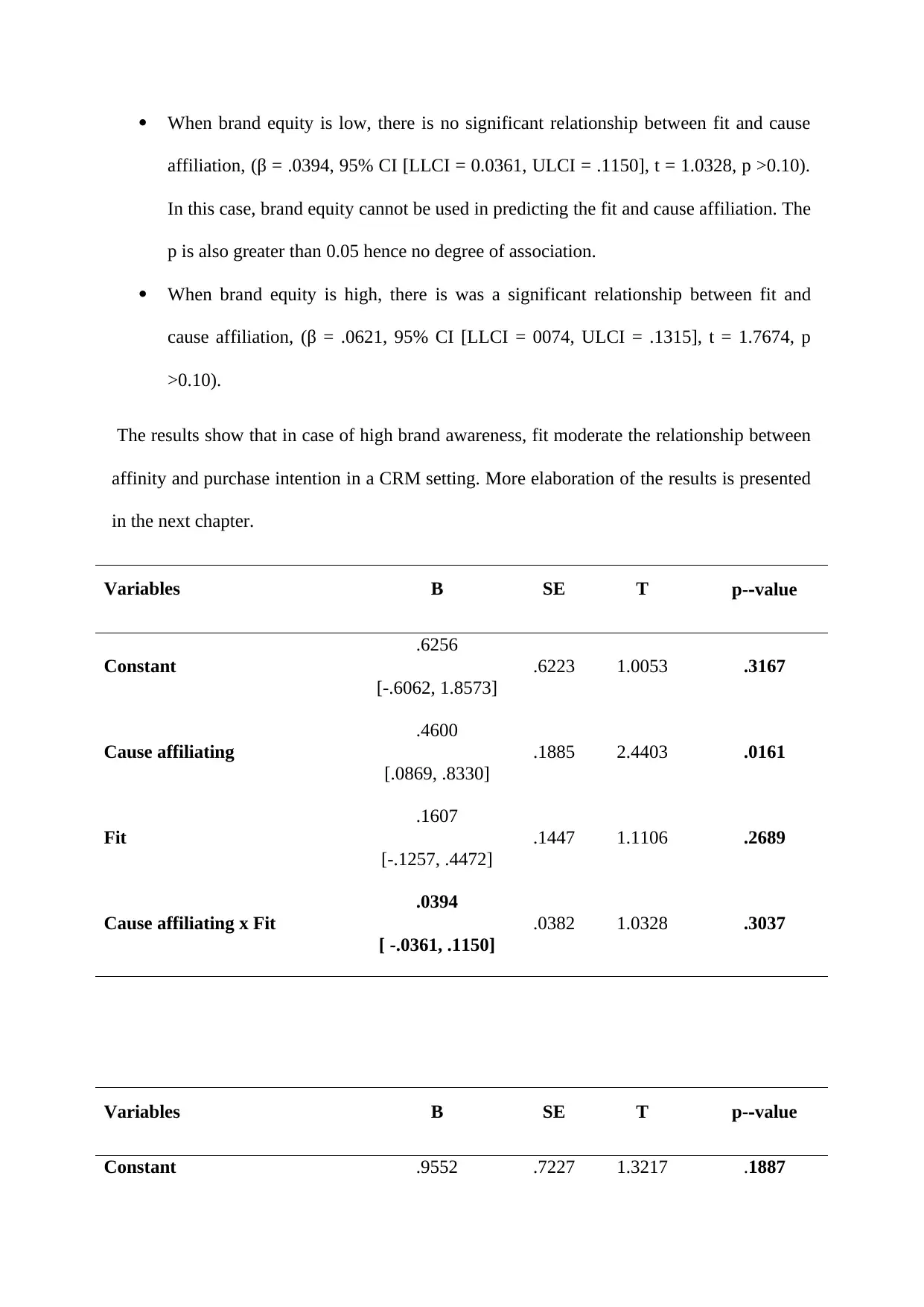
This report presents the results of a statistical analysis focusing on hypothesis testing related to purchase intention within a marketing context. The study employed OLS hierarchical regression and moderation analysis to examine the relationships between variables such as fit, cause affiliation, and brand equity. The analysis included multiple regression to predict purchase intention, with findings indicating a significant relationship between independent variables and the dependent variable. The report details the use of Hayes’ process model for moderation analysis to understand variable interactions, and examines the moderating effects of brand equity. The results support the study's hypothesis, with significant findings and the rejection of the null hypothesis. The report also includes multiple tables displaying statistical values and p-values, and discusses the implications of the findings, including the statistical significance of the regression model. The chapter concludes by summarizing the key findings and alludes to further interpretation and discussion in subsequent chapters.

5.4 Hypothesis Testing
The main effect hypothesis was tested by using OLS hierarchical regression as detailed by
Baron and Kenny (1986). In this work there are multiple studies which can raise the concern
of multicollinearity. It can be a problem interpreting the result accurately as it confounds the
effect of each independent variable on the dependent variable. It can expand the standard
error of the regression coefficient and violate their value. Signs of multicollinearity include
large standard error combined with high R-squared (R2), high correlation between
independent variables (Haire et al., 1998), and high correlation between the estimated
coefficients.
To prevent the problem multicollinearity, (Field, 2009) recommended inspecting the average
scores for each item and inspect the multicollinearity between dependent and the in before
proceeding with multiple regression analysis. Therefore, the regression analysis between
dependent variable (purchase intension) and the independent variables (fit, cause affiliate and
the brand equity) was carried out in this study. The means, standard deviations and pair-wise
correlations among the variables, using SPSS version 20 are presented in the appendix 1of
this work. The results does not list any outstanding regression or correlation between the
values of the predictors i.e. fit, cause affiliate and brand equity. (R > 0.9) (Field, 2009; Hair
et al., 1998; Tabachnick et al., 2001).
In the multiple regression analysis, there are a few important values to consider. The beta
values, which indicate the degree of variance of each independent variable to trust. The R2
value, which identifies how much dose the predictor contributes to the variability in the
outcome. The adjusted R-squared (R2) value, the degree of possibly generalising the results.

It also indicates which variable is the more influential in the model by less than expected by
chance.
To further understand the interaction between the variables, moderation analyses is
conducted. The method used for analysing the moderation effect is Haye’s process model for
moderation analysis was adopted (Hayes, 2012; Preacher & Hayes, 2008). A moderation
analysis extends the exploration of each of the individual predictors in the linear model to
that of the combined effect of two, or more, predictor variables on an outcome (Field, 2009).
A moderation occurs when the relationship between two variables changes as a function of a
third variable. Moderation is tested using a regression in which the outcome is predicted from
a predictor (antecedent dimensions of trust), the moderator (business experience) and the
interaction of these variables (Field, 2009). If the interaction is significant, then moderation is
present and the analysis will be followed up with a simple slopes analysis to examine the
relationship between the predictor and outcome at low, mean and high levels of the
moderator.
5.4.2 Regression Analysis
The multiple regression analysis is an extension of the simple linear regression that can be
used in predicting the value of the dependent variable based on the value of two or more
independent variables. In relation to case, multiple regression analysis will be conducted
since there exists more than one independent variables (i.e. fit, cause affiliation and brand
equity).
The variable we want to predict in our case is the purchase intension which the dependent
variable). Multiple regression analyses thus were conducted to examine the relationship
between the dependent variable (purchase intentions) and independent variables (fit, cause

affiliation and brand equity). Table 5.4.2 below summarizes the descriptive statistics analysis
of the results obtained.
From the results, the regression models of the combined predictors is obtained R2 = .654.
This value indicates a better regression fit for the data. The value of the standard error of the
estimate of the model with the three predictors is 0.903756 which is value close to 1. Thus it
implies a more accuracy of the predictions.
By examining the coefficient table, the constant of the regression model is -0.178. The
coefficients of the predictors are given as; Fit = 0.379, cause affiliate = 0.607 and that of the
brand equity is 0.037. It therefore follows that there exist association between the dependent
and the independent variables. The regression equation for this model is given as;
Purchase intension = -0.178 + 0.379*fit + 0.607*Aflcrs + 0.037*(Brand Equity).
By examining the p-values of all the predictors, both the fit and the affiliation cause has p-
values of 0.000 which are less than 0.05 while the brand equity has p–value of 0.652. With p-
values <0.05 (alpha value), the predictor variables of fit and cause affiliate are significant
because both of their p-values are 0.000.
Model R R Square Adjusted R Square Std. Error of the Estimate
1 .811a .658 .654 .90375
Model Sum of Squares df Mean Square F Sig.
1 Regression 395.666 3 131.889 161.478 .000b

Residual 205.823 252 .817
Total 601.489 255
Model B Std. Error Beta t Sig.
1 (Constant) -.178 .244 -.729 .467
Fit .379 .047 .342 7.986 .000
Afilcsr .607 .045 .578 13.340 .000
BE .037 .081 .017 .452 .652
5.5 Moderating effect and model testing
To interpret the moderating effect and testing the model, we use Hayes’ process by running a
simple moderated regression to examine the interaction effect. The interaction effect occur
when the effect of one variable depends on the value of another variable. This helps in
determining whether the model is good for inferences.
By examining the p-values of the variables, all the p-values in the output table are greater
than 0.05 i.e. p>0.05. This tells us that the interaction effects are not statistically significant.
Consequently, there are relationships between the dependent and the independent variables
since there exist coefficients.

This is Hays model 1, the simplest one. We choose analysis, regression, hays process and we
get this popup:
By testing it, using the regression the model works well since the results shows statistical
significance.
The model below was also tested and it did work. The output is given as shown in the figures
below. The results shows statistical significance as well.
IV. Affinity
with cause
DP. Purchase
intention
Fit
IV. Affinity
with cause
DP. Brand attitude
or maybe PI
Fit BRAND
EQUITY

By considering what is to happen and suppose that the respondent is not aware of either the
target brand, or perhaps, the csr brand, then we might get a different story. It doesn’t make
much sense to consider awareness of the csr brand in our context, though, as we already
check that with affinity for the csr brand. So let’s run our basic model twice; once where
awareness/BE with the target brand is either low or high. I would expect there to be no result
if the target brand awareness is low, but maybe something when respondents are well aware
of the target brand.
We do this by suppressing all data where BEtgt is high, then low.
Model 1, target brand low
awareness/BE (i.e., we don’t expect
a result).
We don’t get a result. Note that
although the lower and upper limits
of the value of the interaction
straddle zero okay (which means
there is an interaction), the interaction is not statistically significant (p= .3037).
The relationship between fit and cause affiliation was examined using Hayes process. The
test was done twice, once with the condition of high brand awareness the second with the
condition low brand awareness. Interpretation of the moderation effect can be undertaken by
examining the simple slopes analysis, as detailed overleaf:

 When brand equity is low, there is no significant relationship between fit and cause
affiliation, (β = .0394, 95% CI [LLCI = 0.0361, ULCI = .1150], t = 1.0328, p >0.10).
In this case, brand equity cannot be used in predicting the fit and cause affiliation. The
p is also greater than 0.05 hence no degree of association.
 When brand equity is high, there is was a significant relationship between fit and
cause affiliation, (β = .0621, 95% CI [LLCI = 0074, ULCI = .1315], t = 1.7674, p
>0.10).
The results show that in case of high brand awareness, fit moderate the relationship between
affinity and purchase intention in a CRM setting. More elaboration of the results is presented
in the next chapter.
Variables B SE T p-‐value
Constant
.6256
[-.6062, 1.8573]
.6223 1.0053 .3167
Cause affiliating
.4600
[.0869, .8330]
.1885 2.4403 .0161
Fit
.1607
[-.1257, .4472]
.1447 1.1106 .2689
Cause affiliating x Fit
.0394
[ -.0361, .1150]
.0382 1.0328 .3037
Variables B SE T p-‐value
Constant .9552 .7227 1.3217 .1887

[-4751, 2.3855]
Cause affiliating
.2642
[.1078, .6363]
.1880 1.4054 .1624
Fit
.2009
[-.0966, .4983]
.1503 1.3364 .1838
Cause affiliating x Fit
.0621
[ -.0074, .1315]
.0351 1.7674 .0796
5.6 Chapter summery
This chapter presented the results of the statistical analysis done leading to the hypothesis
testing. The results supported the hypothesis mentioned in chapter 3. From the findings, the
null hypothesis is rejected. The findings also indicates significance relationship between the
dependent and the independent variables for this study. More interpretation will be presented
in chapter 6 of this work, with the theoretical contraption and directions for future research.