Business Statistics: Data Analysis of Version 1 Product

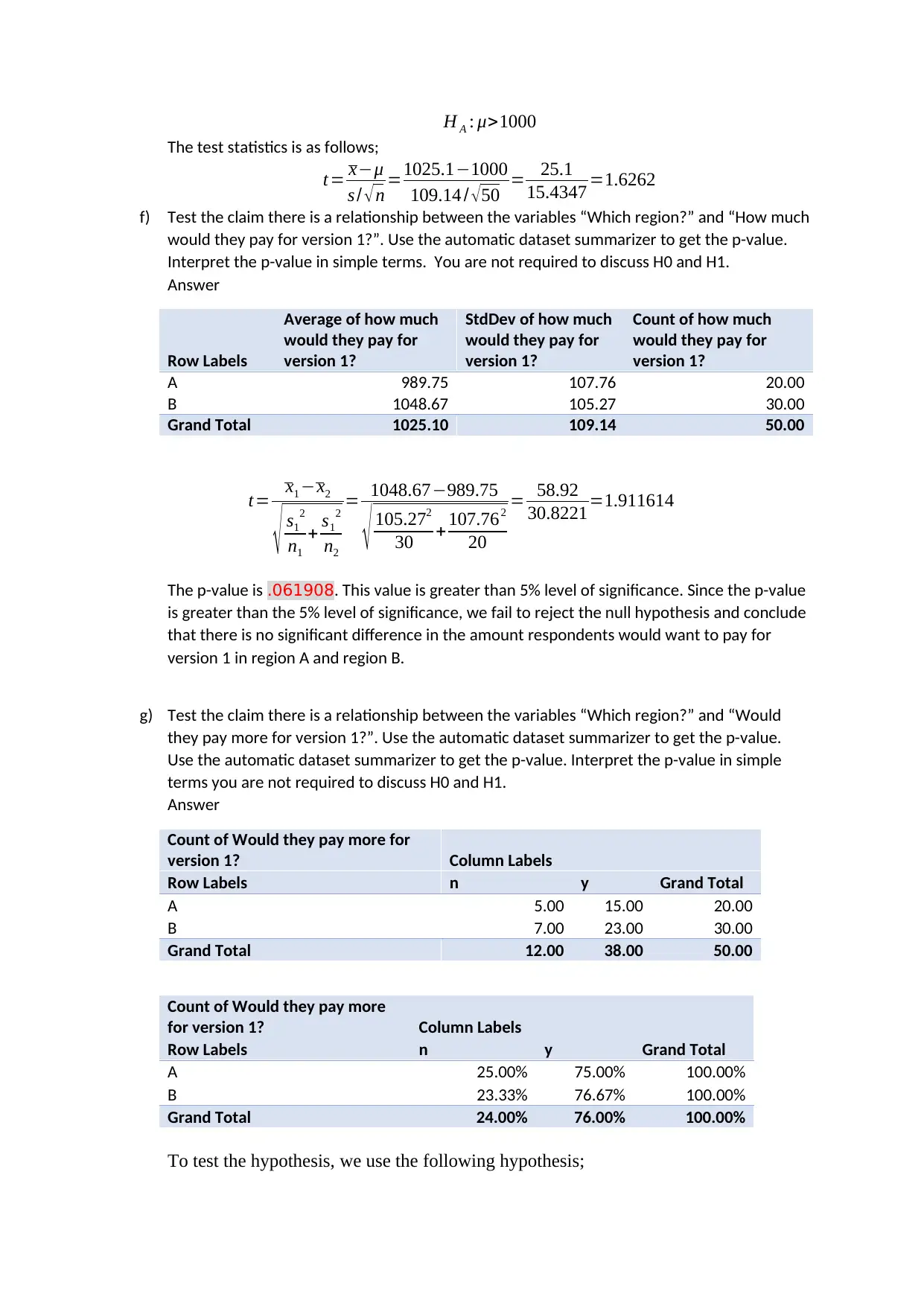
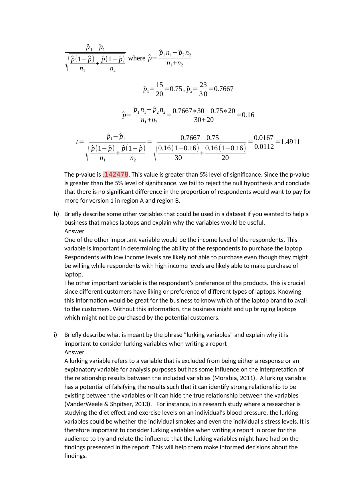
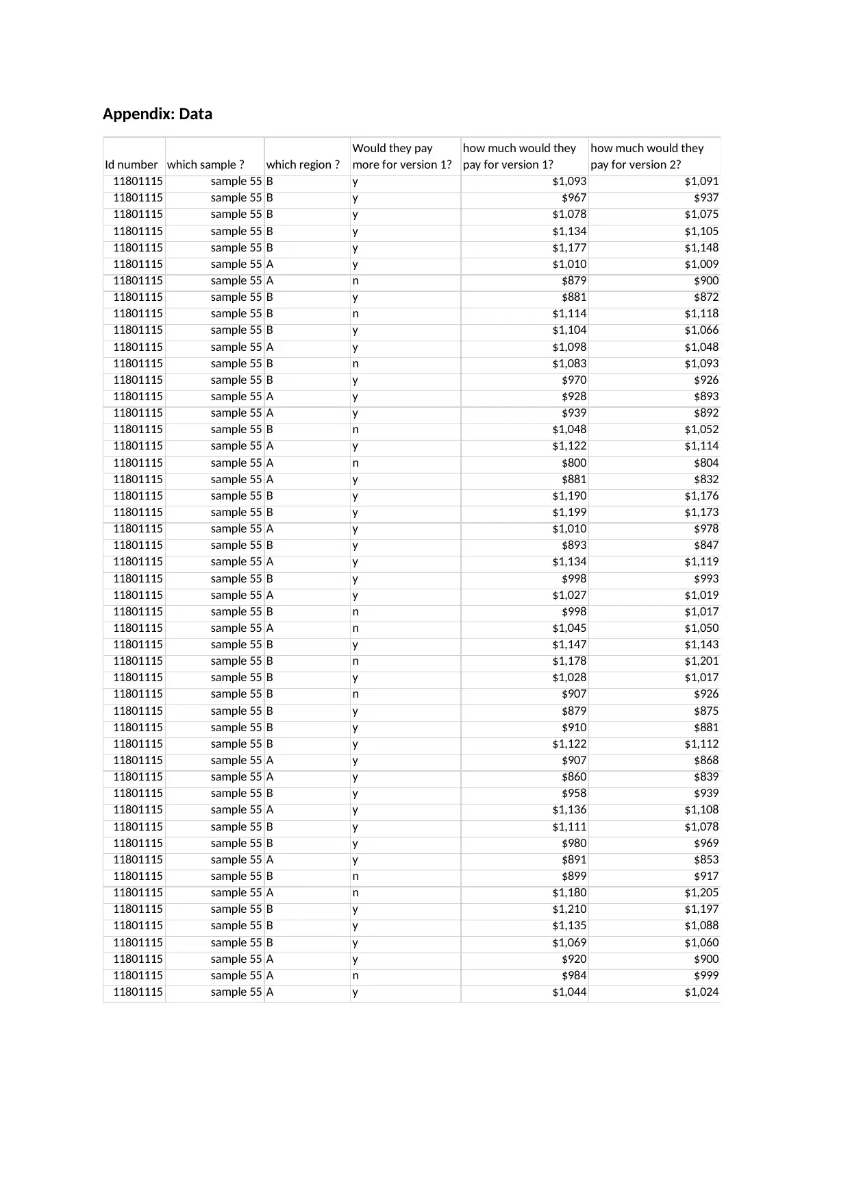
This business statistics report analyzes a customer survey conducted to assess the willingness of respondents in regions A and B to pay for version 1 of a product, given a potential price increase. The report investigates the relationship between region and willingness to pay, as well as the correlation between the price of version 1 and version 2. Key findings include an analysis of average payment amounts, a scatter plot illustrating the relationship between version 1 and version 2 prices, and an examination of the proportion of respondents willing to pay more. The report also includes a 95% confidence interval for the proportion of respondents willing to pay more, a test statistic for the average amount respondents would pay, and p-value interpretations. Furthermore, the report explores the concept of lurking variables and their impact on the analysis, along with recommendations for future data collection and report structuring. The study concludes that there is no evidence to suggest that respondents in regions A and B differ in their willingness to pay for version 1 and that the proportion of respondents willing to pay more does not significantly differ between the regions.

Business Statistics
Student Name:
Instructor Name:
Course Number:
25th May 2019

Executive summary
A business entity is planning to increase the cost of version 1 product. Before increasing the cost,
they conduct a small survey to try and understand the thoughts of the respondents in relation to the
planned hike in price. Results showed that there is no evidence in the amount of money the
respondents in regions A and B are willing to pay for version1. Also, the study shows that the
proportion of respondents willing to pay more for version 1 does not differ for regions A and B.
Background and data set
The ideal behind this survey is to find out whether respondents are willing to have the business
increase the cost of version 1 product.
A sample of 50 customers took part in the survey
Question 1: Which region are you from?
This is a categorical question where respondents were required to either state they come from
region A or region B.
Question 2: Would they pay more for version 1?
This question was also a categorical question where the respondents were required to state whether
they would pay more for version 1. So the answers were either yes (y) or no (n)
Question 3: how much would they pay for version 1?
This is a quantitative variable where the respondents were to state the amount they would want to
pay for version 1.
Question 4: how much would they pay for version 2?
This is a quantitative variable where the respondents were to state the amount they would want to
pay for version 2.
Results and findings
a) Use the automatic dataset summarizer to make a summary that lets you investigate the
relationship between the variables “Which region?” and “How much would they pay for

version 1?”. Paste the summary into the word file. Briefly comment on the relationship
between the variables.
Answer
The table below presents the amount respondents coming from each region would pay for
version 1. Results shows that respondents in region B would pay slightly more for version 1
as compared to respondents in region B. In region A, respondents would want to pay an
average of $989.75 while in region B would want to pay an average of $1048.67 for version
1.
Table 1: Average payment for version 1 in region A and B
Row Labels Average of how much would they pay for version 1?
A 989.75
B 1048.67
Grand Total 1025.10
b) Use the automatic dataset summarizer to make to Make a graph that lets you investigate
the relationship between the variables “How much they would pay for version 1” and “How
much would they pay for version 2” and paste it into the word file . Briefly comment on the
relationship between the variables.
Answer
A scatter plot is presented below to try and investigate the relationship between version 2
payment and version 1 payment. A scatter plot is useful in giving a clear visualization
between two variables (Friendly & Denis, 2015).
Figure 1: Scatter plot of payment for version 2 against payment for version 1
Figure 1 above presents a scatter plot of payment for version 2 against payment for version
1. From the figure, it can be seen that a linear positive relationship exists between payment
for version 2 and payment for version1. This means that an increase in payment for version 2
would result to an increase in the payment for version 1
c) Use the automatic dataset summarizer to make a summary that lets you investigate you
investigate the relationship between the variables “Which region?” and “would you pay

more for version 1” and paste the summary into the word file. Briefly comment on the
relationship between the variables.
Answer
Table 2: Region versus response on paying more
Count of Would they pay more for version 1?
Column
Labels
Row Labels n y Grand Total
A 5.00 15.00 20.00
B 7.00 23.00 30.00
Grand Total 12.00 38.00 50.00
Count of Would they pay more for version
1?
Column
Labels
Row Labels n y Grand Total
A 25.00% 75.00% 100.00%
B 23.33% 76.67% 100.00%
Grand Total 24.00% 76.00% 100.00%
As can be seen from the above tables, 75% (n = 15) of the respondents from region A would
pay more for version 1 while 76.67% (n = 23) of the respondents from region B would pay
more for version 1
d) Find a 95% confidence interval for the variable “would you pay more for version 1”
Answer
We first obtain the proportion of respondents who would pay more for version 1 as follows
^p= x
n =38
50 =0.76
Next we compute the standard error as follows;
σ p= √ p ( 1− p )
n = √ 0.76(1−0.76)
50 = √ 0.1824
50 = √0.003648=0.0604
Next we compute the margin of error as follows;
M . E=Zα /2 σ p =1.96∗0.0604=0.1184
Confidence interval is as follows;
C . I → ^p ± M . E → 0.76 ±0.1184
Lower bound :0.76−0.1184=0.6416
Upper bound :0.76+0.1184=0.8784
From the above computations, we are 95% confident that the true population proportion of
the respondents who would want to pay more for version 1 is between 0.6416 and 0.8784.
e) Find the test stat for testing the claim that people would pay more than $1000 for version 1
on average.
Answer
Average of how much would
they pay for version 1?
StdDev of how much would
they pay for version 1?
1025.10 109.14
The hypothesis we seek to test is as follows;
H0 : μ=1000

H A : μ>1000
The test statistics is as follows;
t= x−μ
s / √ n =1025.1−1000
109.14 / √50 = 25.1
15.4347 =1.6262
f) Test the claim there is a relationship between the variables “Which region?” and “How much
would they pay for version 1?”. Use the automatic dataset summarizer to get the p-value.
Interpret the p-value in simple terms. You are not required to discuss H0 and H1.
Answer
Row Labels
Average of how much
would they pay for
version 1?
StdDev of how much
would they pay for
version 1?
Count of how much
would they pay for
version 1?
A 989.75 107.76 20.00
B 1048.67 105.27 30.00
Grand Total 1025.10 109.14 50.00
t= x1 −x2
√ s1
2
n1
+ s1
2
n2
= 1048.67−989.75
√ 105.272
30 + 107.762
20
= 58.92
30.8221=1.911614
The p-value is .061908. This value is greater than 5% level of significance. Since the p-value
is greater than the 5% level of significance, we fail to reject the null hypothesis and conclude
that there is no significant difference in the amount respondents would want to pay for
version 1 in region A and region B.
g) Test the claim there is a relationship between the variables “Which region?” and “Would
they pay more for version 1?”. Use the automatic dataset summarizer to get the p-value.
Use the automatic dataset summarizer to get the p-value. Interpret the p-value in simple
terms you are not required to discuss H0 and H1.
Answer
Count of Would they pay more for
version 1? Column Labels
Row Labels n y Grand Total
A 5.00 15.00 20.00
B 7.00 23.00 30.00
Grand Total 12.00 38.00 50.00
Count of Would they pay more
for version 1? Column Labels
Row Labels n y Grand Total
A 25.00% 75.00% 100.00%
B 23.33% 76.67% 100.00%
Grand Total 24.00% 76.00% 100.00%
To test the hypothesis, we use the following hypothesis;

^p1− ^p1
√ ^p(1− ^p)
n1
+ ^p(1− ^p)
n2
where ^p= ^p1 n1− ^p2 n2
n1 +n2
^p1= 15
20 =0.75 , ^p2= 23
3 0 =0.7667
^p= ^p1 n1− ^p2 n2
n1 +n2
=0.7667∗30−0.75∗20
30+20 =0.16
t= ^p1− ^p1
√ ^p(1− ^p)
n1
+ ^p(1− ^p)
n2
= 0.7667−0.75
√ 0.16( 1−0.16)
30 + 0.16 (1−0.16)
20
=0.0167
0.0112 =1.4911
The p-value is .142478. This value is greater than 5% level of significance. Since the p-value
is greater than the 5% level of significance, we fail to reject the null hypothesis and conclude
that there is no significant difference in the proportion of respondents would want to pay for
more for version 1 in region A and region B.
h) Briefly describe some other variables that could be used in a dataset if you wanted to help a
business that makes laptops and explain why the variables would be useful.
Answer
One of the other important variable would be the income level of the respondents. This
variable is important in determining the ability of the respondents to purchase the laptop
Respondents with low income levels are likely not able to purchase even though they might
be willing while respondents with high income levels are likely able to make purchase of
laptop.
The other important variable is the respondent’s preference of the products. This is crucial
since different customers have liking or preference of different types of laptops. Knowing
this information would be great for the business to know which of the laptop brand to avail
to the customers. Without this information, the business might end up bringing laptops
which might not be purchased by the potential customers.
i) Briefly describe what is meant by the phrase “lurking variables” and explain why it is
important to consider lurking variables when writing a report
Answer
A lurking variable refers to a variable that is excluded from being either a response or an
explanatory variable for analysis purposes but has some influence on the interpretation of
the relationship results between the included variables (Morabia, 2011). A lurking variable
has a potential of falsifying the results such that it can identify strong relationship to be
existing between the variables or it can hide the true relationship between the variables
(VanderWeele & Shpitser, 2013). For instance, in a research study where a researcher is
studying the diet effect and exercise levels on an individual’s blood pressure, the lurking
variables could be whether the individual smokes and even the individual’s stress levels. It is
therefore important to consider lurking variables when writing a report in order for the
audience to try and relate the influence that the lurking variables might have had on the
findings presented in the report. This will help them make informed decisions about the
findings.

j) Briefly describe how you would make a report that uses the information from at least 5 of
the previous parts of the assignment, the previous parts of the assignment are parts (a),(b),
(c),(d),(e),(f),(g),(h),(i) given above
Answer
To make a report that uses the information from at least 5 of the previous parts of the
assignment, we need to understand the hypothesis test that each of the sections is trying to
answer. When we know the hypothesis being answered by each section then we can identify
which of the sections to include in the final report. The objective of the final report should
also be well known and articulated so that the sections are just used to answer the
objectives.
Conclusion
There is no evidence in the amount of money the respondents in regions A and B are willing to pay
for version1. Also, the study shows that the proportion of respondents willing to pay more for
version 1 does not differ for regions A and B.

References
Friendly, M. & Denis, D., 2015. The early origins and development of the scatterplot.
Journal of the History of the Behavioral Sciences, 41(2), p. 103–130.
Morabia, A., 2011. History of the modern epidemiological concept of confounding. Journal
of Epidemiology and Community Health, 65(4), p. 297–300.
VanderWeele, T. & Shpitser, I., 2013. On the definition of a confounder. Annals of Statistics,
41(1), p. 196–220.

Appendix: Data
Id number which sample ? which region ?
Would they pay
more for version 1?
how much would they
pay for version 1?
how much would they
pay for version 2?
11801115 sample 55 B y $1,093 $1,091
11801115 sample 55 B y $967 $937
11801115 sample 55 B y $1,078 $1,075
11801115 sample 55 B y $1,134 $1,105
11801115 sample 55 B y $1,177 $1,148
11801115 sample 55 A y $1,010 $1,009
11801115 sample 55 A n $879 $900
11801115 sample 55 B y $881 $872
11801115 sample 55 B n $1,114 $1,118
11801115 sample 55 B y $1,104 $1,066
11801115 sample 55 A y $1,098 $1,048
11801115 sample 55 B n $1,083 $1,093
11801115 sample 55 B y $970 $926
11801115 sample 55 A y $928 $893
11801115 sample 55 A y $939 $892
11801115 sample 55 B n $1,048 $1,052
11801115 sample 55 A y $1,122 $1,114
11801115 sample 55 A n $800 $804
11801115 sample 55 A y $881 $832
11801115 sample 55 B y $1,190 $1,176
11801115 sample 55 B y $1,199 $1,173
11801115 sample 55 A y $1,010 $978
11801115 sample 55 B y $893 $847
11801115 sample 55 A y $1,134 $1,119
11801115 sample 55 B y $998 $993
11801115 sample 55 A y $1,027 $1,019
11801115 sample 55 B n $998 $1,017
11801115 sample 55 A n $1,045 $1,050
11801115 sample 55 B y $1,147 $1,143
11801115 sample 55 B n $1,178 $1,201
11801115 sample 55 B y $1,028 $1,017
11801115 sample 55 B n $907 $926
11801115 sample 55 B y $879 $875
11801115 sample 55 B y $910 $881
11801115 sample 55 B y $1,122 $1,112
11801115 sample 55 A y $907 $868
11801115 sample 55 A y $860 $839
11801115 sample 55 B y $958 $939
11801115 sample 55 A y $1,136 $1,108
11801115 sample 55 B y $1,111 $1,078
11801115 sample 55 B y $980 $969
11801115 sample 55 A y $891 $853
11801115 sample 55 B n $899 $917
11801115 sample 55 A n $1,180 $1,205
11801115 sample 55 B y $1,210 $1,197
11801115 sample 55 B y $1,135 $1,088
11801115 sample 55 B y $1,069 $1,060
11801115 sample 55 A y $920 $900
11801115 sample 55 A n $984 $999
11801115 sample 55 A y $1,044 $1,024