University of Westminster Data Analysis Assignment - 7ECON001W
VerifiedAdded on 2022/08/23
|26
|3427
|25
Homework Assignment
AI Summary
This document presents a comprehensive solution to a data analysis assignment for the 7ECON001W course at the University of Westminster's Westminster Business School. The assignment covers a wide range of econometrics topics, including regression analysis, hypothesis testing, and the identification and correction of statistical issues. The solution begins with an analysis of a regression model, interpreting coefficients, and assessing statistical significance using t-tests and p-values. It then delves into the overall significance of the model using the F-test, and explores potential multicollinearity problems. The solution also addresses heteroscedasticity, employing residual plots, the White test, and generalized least squares (GLS) methods to correct for it. Furthermore, the assignment examines serial autocorrelation, using correlograms and the Breusch-Godfrey test to assess its presence, and then discusses the effects of autocorrelation on the OLS estimators. Finally, the solution provides results from White's autocorrelation and heteroscedasticity consistent standard errors and the Cochrane-Orcutt estimation to resolve these econometric issues. The assignment provides a detailed, step-by-step approach to solving the problems, along with interpretations of the results and relevant EViews outputs.
Running head: DATA ANALYSIS
Data Analysis
Name of the Student
Name of the University
Course ID
Data Analysis
Name of the Student
Name of the University
Course ID
Paraphrase This Document
Need a fresh take? Get an instant paraphrase of this document with our AI Paraphraser
1DATA ANALYSIS
Table of Contents
Question 1........................................................................................................................................2
Question a....................................................................................................................................2
Question b....................................................................................................................................3
Question 2........................................................................................................................................4
Question a....................................................................................................................................4
Question b....................................................................................................................................4
Question 3........................................................................................................................................5
Question 4........................................................................................................................................6
Question a....................................................................................................................................6
Question b....................................................................................................................................7
Question 5........................................................................................................................................7
Question b....................................................................................................................................8
Question 6........................................................................................................................................9
Question a....................................................................................................................................9
Question b..................................................................................................................................10
Question 7......................................................................................................................................11
Question 8......................................................................................................................................11
Question a..................................................................................................................................12
Question b..................................................................................................................................13
Question 9......................................................................................................................................13
Question a..................................................................................................................................13
Question b..................................................................................................................................14
Question 10....................................................................................................................................15
Question 11....................................................................................................................................16
Question a..................................................................................................................................16
Question b..................................................................................................................................17
Question 12....................................................................................................................................18
Question 13....................................................................................................................................20
Question 14....................................................................................................................................20
Question 15....................................................................................................................................21
Question 16....................................................................................................................................22
References......................................................................................................................................23
2DATA ANALYSIS
Question 1
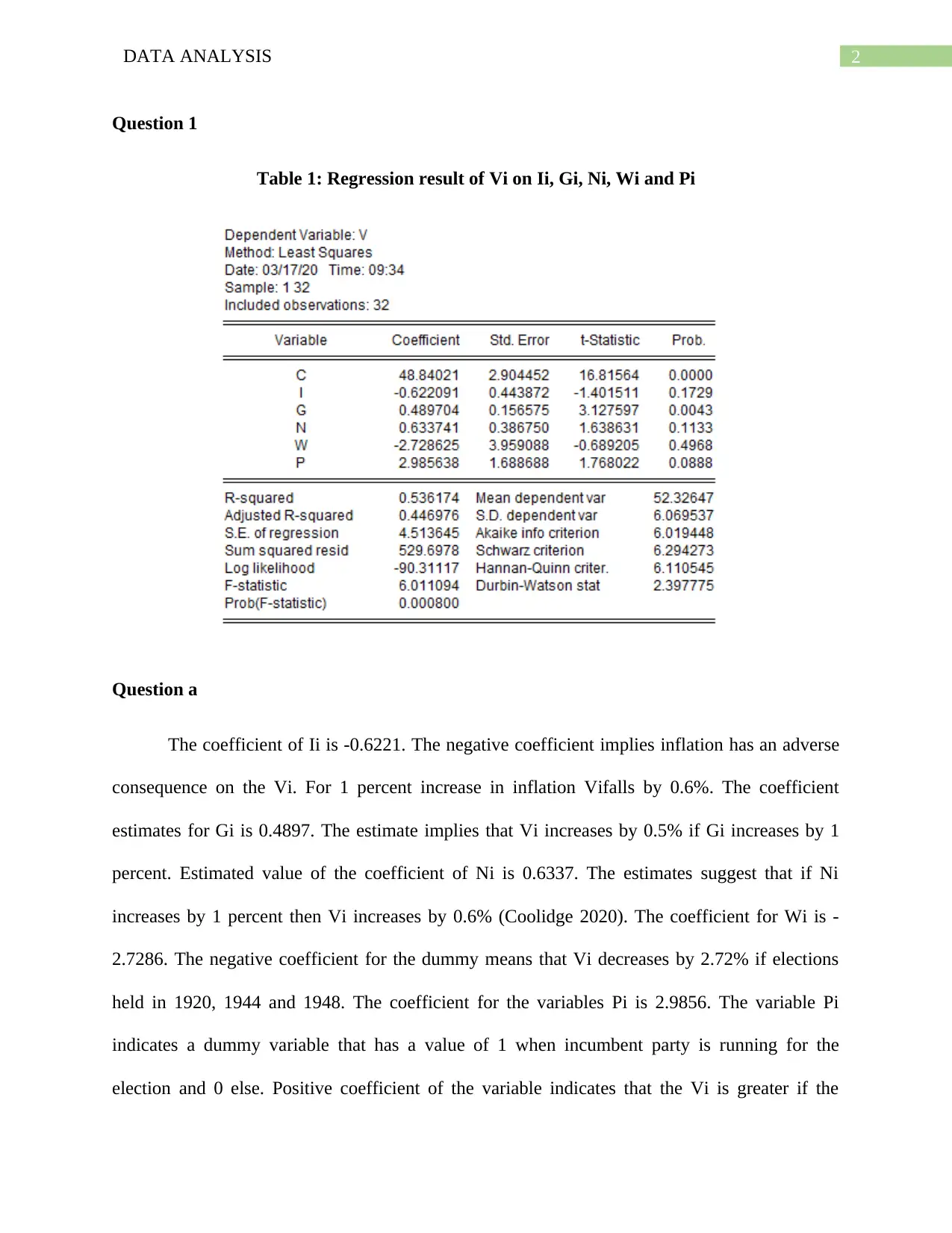
Table 1: Regression result of Vi on Ii, Gi, Ni, Wi and Pi
Question a
The coefficient of Ii is -0.6221. The negative coefficient implies inflation has an adverse
consequence on the Vi. For 1 percent increase in inflation Vifalls by 0.6%. The coefficient
estimates for Gi is 0.4897. The estimate implies that Vi increases by 0.5% if Gi increases by 1
percent. Estimated value of the coefficient of Ni is 0.6337. The estimates suggest that if Ni
increases by 1 percent then Vi increases by 0.6% (Coolidge 2020). The coefficient for Wi is -
2.7286. The negative coefficient for the dummy means that Vi decreases by 2.72% if elections
held in 1920, 1944 and 1948. The coefficient for the variables Pi is 2.9856. The variable Pi
indicates a dummy variable that has a value of 1 when incumbent party is running for the
election and 0 else. Positive coefficient of the variable indicates that the Vi is greater if the
Question 1
Table 1: Regression result of Vi on Ii, Gi, Ni, Wi and Pi
Question a
The coefficient of Ii is -0.6221. The negative coefficient implies inflation has an adverse
consequence on the Vi. For 1 percent increase in inflation Vifalls by 0.6%. The coefficient
estimates for Gi is 0.4897. The estimate implies that Vi increases by 0.5% if Gi increases by 1
percent. Estimated value of the coefficient of Ni is 0.6337. The estimates suggest that if Ni
increases by 1 percent then Vi increases by 0.6% (Coolidge 2020). The coefficient for Wi is -
2.7286. The negative coefficient for the dummy means that Vi decreases by 2.72% if elections
held in 1920, 1944 and 1948. The coefficient for the variables Pi is 2.9856. The variable Pi
indicates a dummy variable that has a value of 1 when incumbent party is running for the
election and 0 else. Positive coefficient of the variable indicates that the Vi is greater if the
⊘ This is a preview!⊘
Do you want full access?
Subscribe today to unlock all pages.
Trusted by 1+ million students worldwide
3DATA ANALYSIS
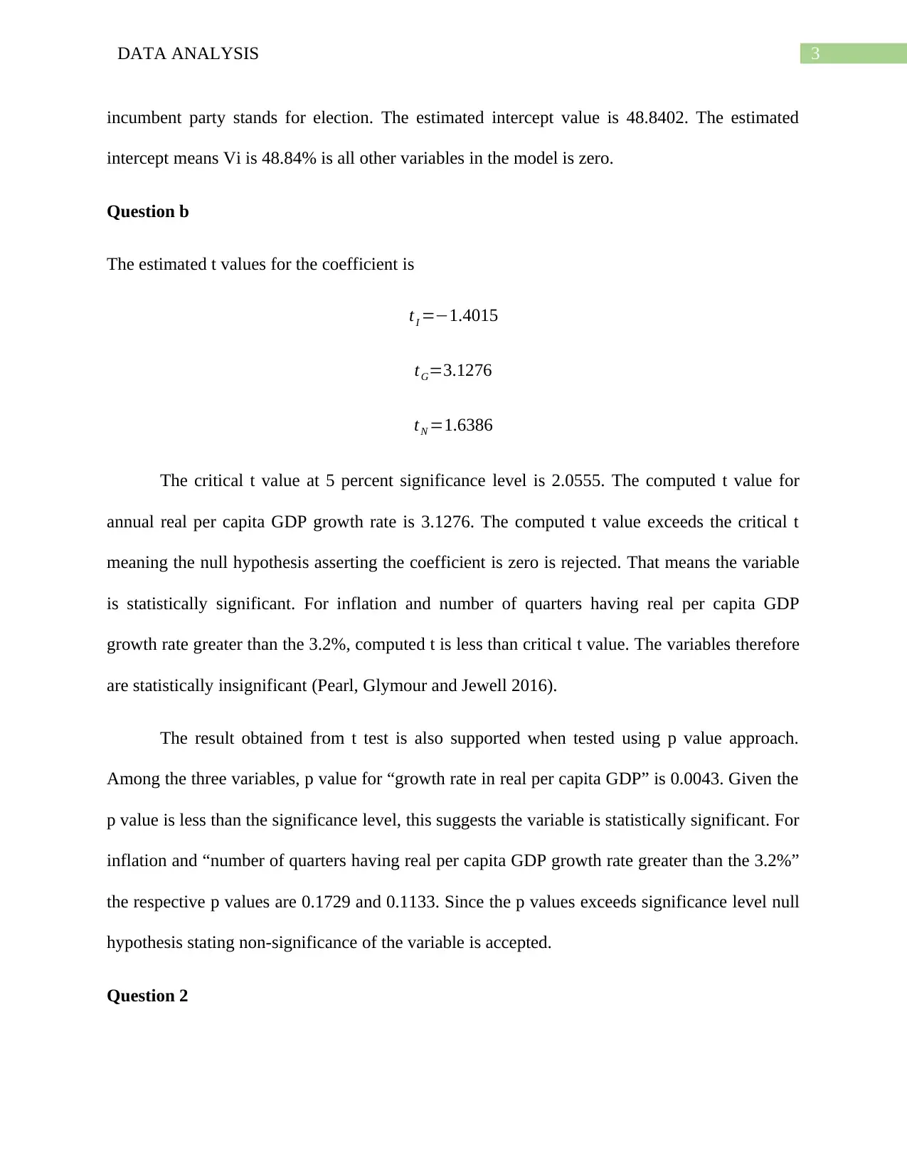
incumbent party stands for election. The estimated intercept value is 48.8402. The estimated
intercept means Vi is 48.84% is all other variables in the model is zero.
Question b
The estimated t values for the coefficient is
tI =−1.4015
tG=3.1276
tN =1.6386
The critical t value at 5 percent significance level is 2.0555. The computed t value for
annual real per capita GDP growth rate is 3.1276. The computed t value exceeds the critical t
meaning the null hypothesis asserting the coefficient is zero is rejected. That means the variable
is statistically significant. For inflation and number of quarters having real per capita GDP
growth rate greater than the 3.2%, computed t is less than critical t value. The variables therefore
are statistically insignificant (Pearl, Glymour and Jewell 2016).
The result obtained from t test is also supported when tested using p value approach.
Among the three variables, p value for “growth rate in real per capita GDP” is 0.0043. Given the
p value is less than the significance level, this suggests the variable is statistically significant. For
inflation and “number of quarters having real per capita GDP growth rate greater than the 3.2%”
the respective p values are 0.1729 and 0.1133. Since the p values exceeds significance level null
hypothesis stating non-significance of the variable is accepted.
Question 2
Paraphrase This Document
Need a fresh take? Get an instant paraphrase of this document with our AI Paraphraser
4DATA ANALYSIS
For overall significance F test is used. The computed F value for the model is obtained as
6.0110. The critical F value corresponding to alpha value of 0.05 is 2.5868. The computed F
value exceeds the critical F vale suggesting rejection of null hypothesis that all the slope
coefficients are equal zero. This means that the independent variables are significant jointly. The
Result can be verified using the associated p value of the statistics (Robertson and McCloskey
2019). The p value associated with F statistics is 0.008. Given the p value is less than chosen
significance level at 5% the null hypothesis that the independent variables are jointly
insignificant is rejected. The independent variables therefore are jointly significant.
Other factors that might affect Vi are publicity campaign, expenditures on social
program, expenditure made by the incumbent party to enhance facilities such as health care,
availability of drinking water, education and others.
Question a
Goodness of fit of the model can be examined from the R square value. The obtained R
square value is 0.54. That means the variables considered in the model accounts for 54 percent
variation in Vi. The R square value suggests that the model is a moderately good fit.
Question b
The result of F test shows that the model has overall significance meaning all the
independent variables are significant jointly. However, whenever testing for individual
significance of the regression coefficient using t-tests, the obtained result indicates only growth
rate is statistically significant while all others are insignificant. This is possible when
independent variables are correlated (Schroeder, Sjoquist and Stephan 2016). Under such
circumstances the model can be improved by dropping some of the insignificant variables.
5DATA ANALYSIS
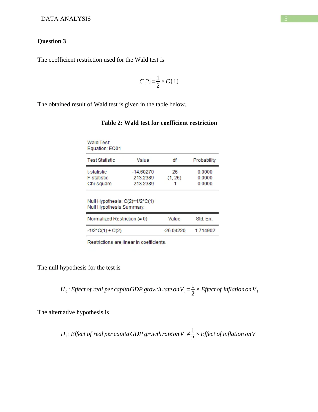
Question 3
The coefficient restriction used for the Wald test is
C ( 2 ) =1
2 × C(1)
The obtained result of Wald test is given in the table below.
Table 2: Wald test for coefficient restriction
The null hypothesis for the test is
H0 : Effect of real per capitaGDP growth rate onV i =1
2 × Effect of inflation on V i
The alternative hypothesis is
H1 : Effect of real per capita GDP growthrate on V i ≠ 1
2 × Effect of inflation onV i
⊘ This is a preview!⊘
Do you want full access?
Subscribe today to unlock all pages.
Trusted by 1+ million students worldwide
6DATA ANALYSIS
The p value of the test statistics result is 0.0000. The p value is smaller compared to the
significance level suggesting rejection of null hypothesis that the coefficient restriction holds.
Therefore, effect of extra 1% “real per capita GDP growth rate” on “percentage share of popular
vote won by the incumbent party” does not equal to half of the effect of extra 1% inflation on the
same.
Question 4
Question a
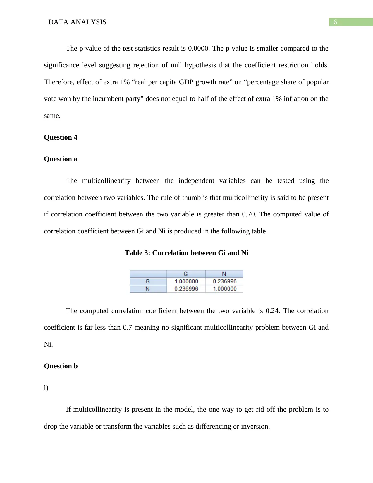
The multicollinearity between the independent variables can be tested using the
correlation between two variables. The rule of thumb is that multicollinerity is said to be present
if correlation coefficient between the two variable is greater than 0.70. The computed value of
correlation coefficient between Gi and Ni is produced in the following table.
Table 3: Correlation between Gi and Ni
The computed correlation coefficient between the two variable is 0.24. The correlation
coefficient is far less than 0.7 meaning no significant multicollinearity problem between Gi and
Ni.
Question b
i)
If multicollinearity is present in the model, the one way to get rid-off the problem is to
drop the variable or transform the variables such as differencing or inversion.
The p value of the test statistics result is 0.0000. The p value is smaller compared to the
significance level suggesting rejection of null hypothesis that the coefficient restriction holds.
Therefore, effect of extra 1% “real per capita GDP growth rate” on “percentage share of popular
vote won by the incumbent party” does not equal to half of the effect of extra 1% inflation on the
same.
Question 4
Question a
The multicollinearity between the independent variables can be tested using the
correlation between two variables. The rule of thumb is that multicollinerity is said to be present
if correlation coefficient between the two variable is greater than 0.70. The computed value of
correlation coefficient between Gi and Ni is produced in the following table.
Table 3: Correlation between Gi and Ni
The computed correlation coefficient between the two variable is 0.24. The correlation
coefficient is far less than 0.7 meaning no significant multicollinearity problem between Gi and
Ni.
Question b
i)
If multicollinearity is present in the model, the one way to get rid-off the problem is to
drop the variable or transform the variables such as differencing or inversion.
Paraphrase This Document
Need a fresh take? Get an instant paraphrase of this document with our AI Paraphraser
7DATA ANALYSIS
ii) In the presence of multicollinerity, standard error of the regression coefficient may become
very large. Large value standard errors result in a relatively smaller value of the t statistics.
Based on smaller t value researchers have a tendency to accept null hypothesis. This in turn
increases the possibility of occurring type II error (Daoud 2017). The presence of
multicollinearity though gives BLUE and consistent OLS estimator, it may result in
misspecification of the model.
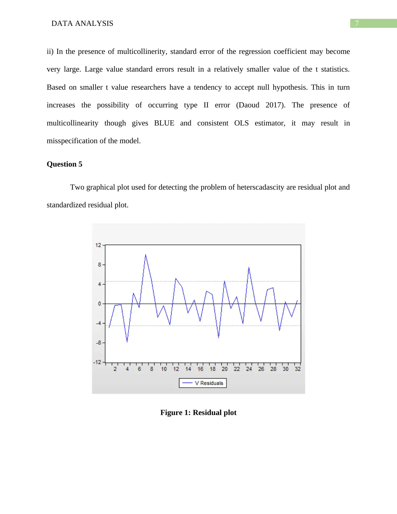
Question 5
Two graphical plot used for detecting the problem of heterscadascity are residual plot and
standardized residual plot.
Figure 1: Residual plot
ii) In the presence of multicollinerity, standard error of the regression coefficient may become
very large. Large value standard errors result in a relatively smaller value of the t statistics.
Based on smaller t value researchers have a tendency to accept null hypothesis. This in turn
increases the possibility of occurring type II error (Daoud 2017). The presence of
multicollinearity though gives BLUE and consistent OLS estimator, it may result in
misspecification of the model.
Question 5
Two graphical plot used for detecting the problem of heterscadascity are residual plot and
standardized residual plot.
Figure 1: Residual plot
8DATA ANALYSIS
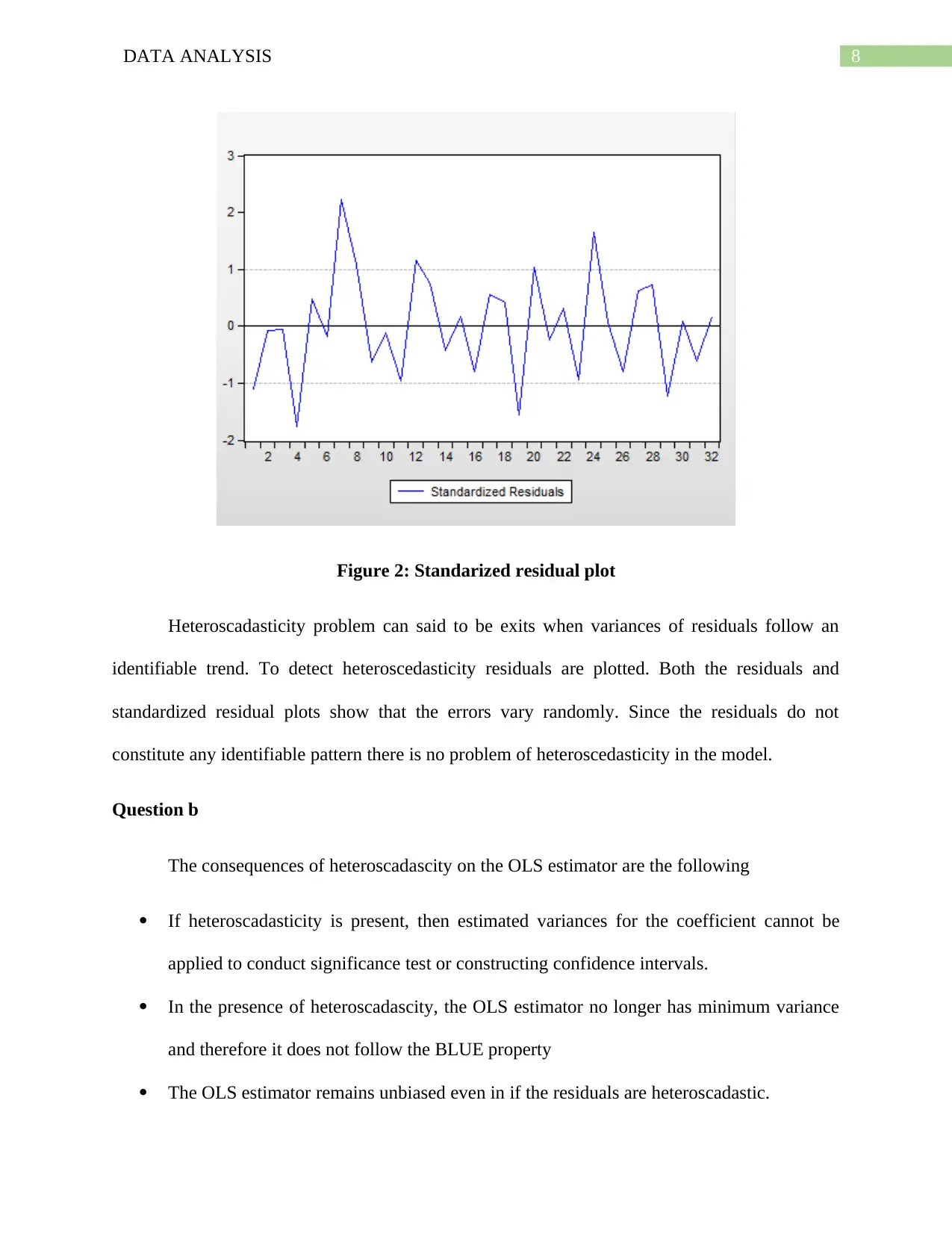
Figure 2: Standarized residual plot
Heteroscadasticity problem can said to be exits when variances of residuals follow an
identifiable trend. To detect heteroscedasticity residuals are plotted. Both the residuals and
standardized residual plots show that the errors vary randomly. Since the residuals do not
constitute any identifiable pattern there is no problem of heteroscedasticity in the model.
Question b
The consequences of heteroscadascity on the OLS estimator are the following
If heteroscadasticity is present, then estimated variances for the coefficient cannot be
applied to conduct significance test or constructing confidence intervals.
In the presence of heteroscadascity, the OLS estimator no longer has minimum variance
and therefore it does not follow the BLUE property
The OLS estimator remains unbiased even in if the residuals are heteroscadastic.
⊘ This is a preview!⊘
Do you want full access?
Subscribe today to unlock all pages.
Trusted by 1+ million students worldwide
9DATA ANALYSIS
If heteroscadascity is present, OLS estimator gives inefficient forecasting because of
larger variance of the coefficient.
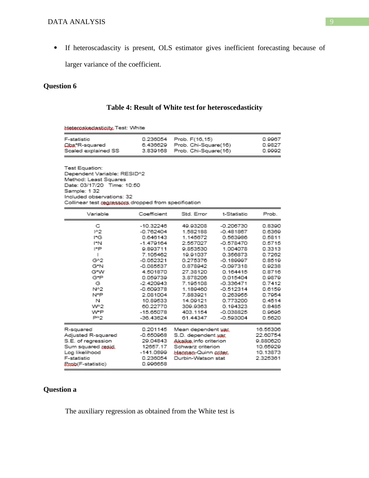
Question 6
Table 4: Result of White test for heteroscedasticity
Question a
The auxiliary regression as obtained from the White test is
If heteroscadascity is present, OLS estimator gives inefficient forecasting because of
larger variance of the coefficient.
Question 6
Table 4: Result of White test for heteroscedasticity
Question a
The auxiliary regression as obtained from the White test is
Paraphrase This Document
Need a fresh take? Get an instant paraphrase of this document with our AI Paraphraser
10DATA ANALYSIS
ei
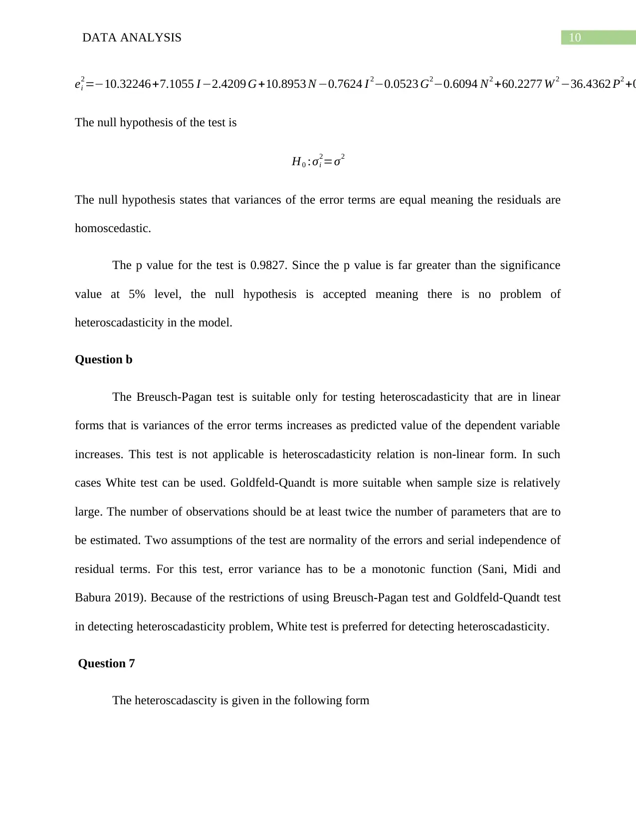
2=−10.32246+7.1055 I −2.4209 G+10.8953 N −0.7624 I 2−0.0523 G2−0.6094 N2 +60.2277 W 2 −36.4362 P2 +0
The null hypothesis of the test is
H0 :σi
2=σ2
The null hypothesis states that variances of the error terms are equal meaning the residuals are
homoscedastic.
The p value for the test is 0.9827. Since the p value is far greater than the significance
value at 5% level, the null hypothesis is accepted meaning there is no problem of
heteroscadasticity in the model.
Question b
The Breusch-Pagan test is suitable only for testing heteroscadasticity that are in linear
forms that is variances of the error terms increases as predicted value of the dependent variable
increases. This test is not applicable is heteroscadasticity relation is non-linear form. In such
cases White test can be used. Goldfeld-Quandt is more suitable when sample size is relatively
large. The number of observations should be at least twice the number of parameters that are to
be estimated. Two assumptions of the test are normality of the errors and serial independence of
residual terms. For this test, error variance has to be a monotonic function (Sani, Midi and
Babura 2019). Because of the restrictions of using Breusch-Pagan test and Goldfeld-Quandt test
in detecting heteroscadasticity problem, White test is preferred for detecting heteroscadasticity.
Question 7
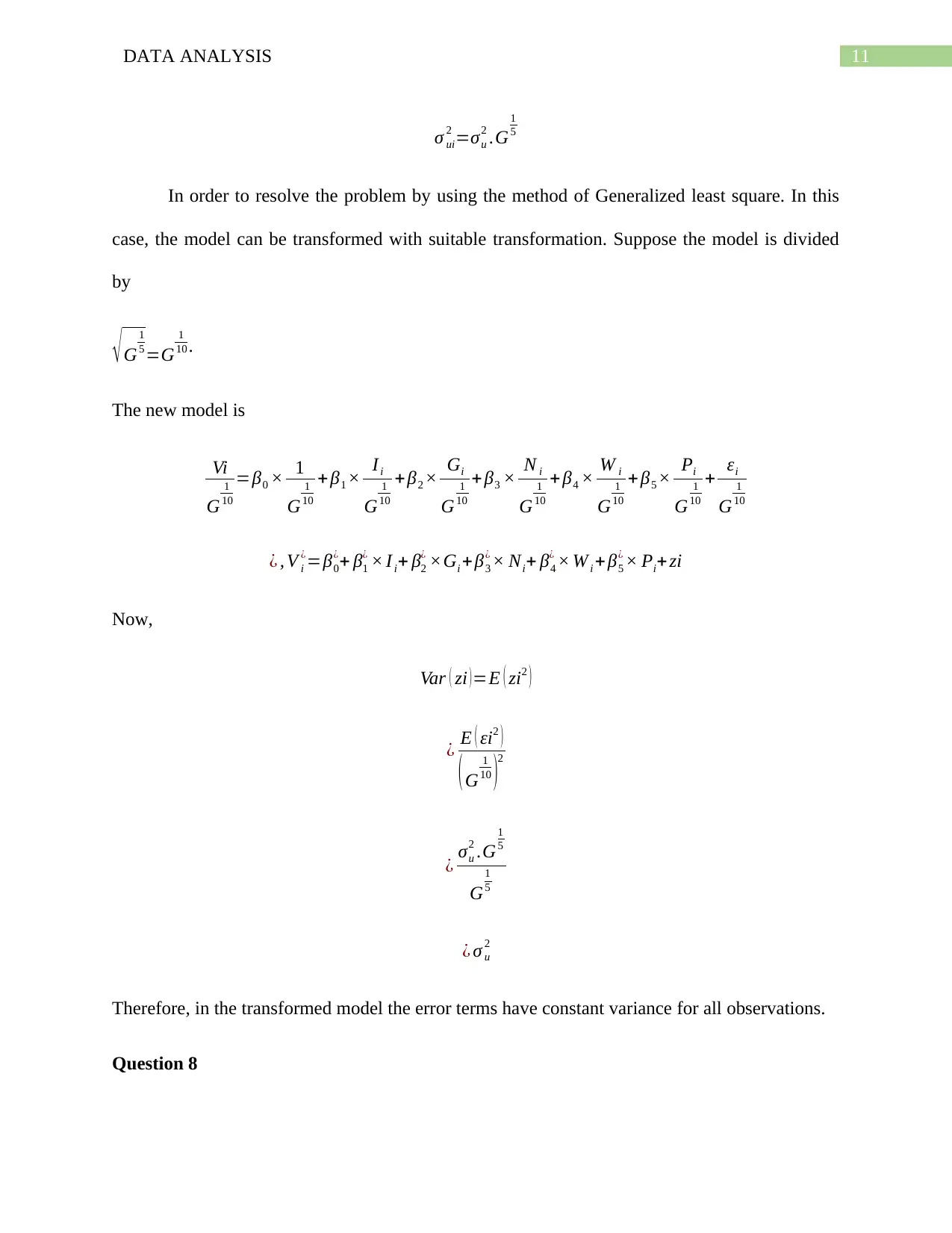
The heteroscadascity is given in the following form
ei
2=−10.32246+7.1055 I −2.4209 G+10.8953 N −0.7624 I 2−0.0523 G2−0.6094 N2 +60.2277 W 2 −36.4362 P2 +0
The null hypothesis of the test is
H0 :σi
2=σ2
The null hypothesis states that variances of the error terms are equal meaning the residuals are
homoscedastic.
The p value for the test is 0.9827. Since the p value is far greater than the significance
value at 5% level, the null hypothesis is accepted meaning there is no problem of
heteroscadasticity in the model.
Question b
The Breusch-Pagan test is suitable only for testing heteroscadasticity that are in linear
forms that is variances of the error terms increases as predicted value of the dependent variable
increases. This test is not applicable is heteroscadasticity relation is non-linear form. In such
cases White test can be used. Goldfeld-Quandt is more suitable when sample size is relatively
large. The number of observations should be at least twice the number of parameters that are to
be estimated. Two assumptions of the test are normality of the errors and serial independence of
residual terms. For this test, error variance has to be a monotonic function (Sani, Midi and
Babura 2019). Because of the restrictions of using Breusch-Pagan test and Goldfeld-Quandt test
in detecting heteroscadasticity problem, White test is preferred for detecting heteroscadasticity.
Question 7
The heteroscadascity is given in the following form
11DATA ANALYSIS
σ ui
2 =σu
2 .G
1
5
In order to resolve the problem by using the method of Generalized least square. In this
case, the model can be transformed with suitable transformation. Suppose the model is divided
by
√G
1
5 =G
1
10 .
The new model is
Vi
G
1
10
=β0 × 1
G
1
10
+ β1 × Ii
G
1
10
+ β2 × Gi
G
1
10
+β3 × N i
G
1
10
+ β4 × W i
G
1
10
+ β5 × Pi
G
1
10
+ εi
G
1
10
¿ , V i
¿=β0
¿+ β1
¿ × I i+ β2
¿ ×Gi +β3
¿ × Ni+ β4
¿ × W i + β5
¿ × Pi+ zi
Now,
Var ( zi )=E ( zi2 )
¿ E ( εi2 )
(G
1
10 )2
¿ σu
2 .G
1
5
G
1
5
¿ σ u
2
Therefore, in the transformed model the error terms have constant variance for all observations.
Question 8
⊘ This is a preview!⊘
Do you want full access?
Subscribe today to unlock all pages.
Trusted by 1+ million students worldwide
1 out of 26


Your All-in-One AI-Powered Toolkit for Academic Success.
+13062052269
info@desklib.com
Available 24*7 on WhatsApp / Email
![[object Object]](/_next/static/media/star-bottom.7253800d.svg)
Unlock your academic potential
Copyright © 2020–2026 A2Z Services. All Rights Reserved. Developed and managed by ZUCOL.