Data Analysis and Business Intelligence Report: Superstore Data

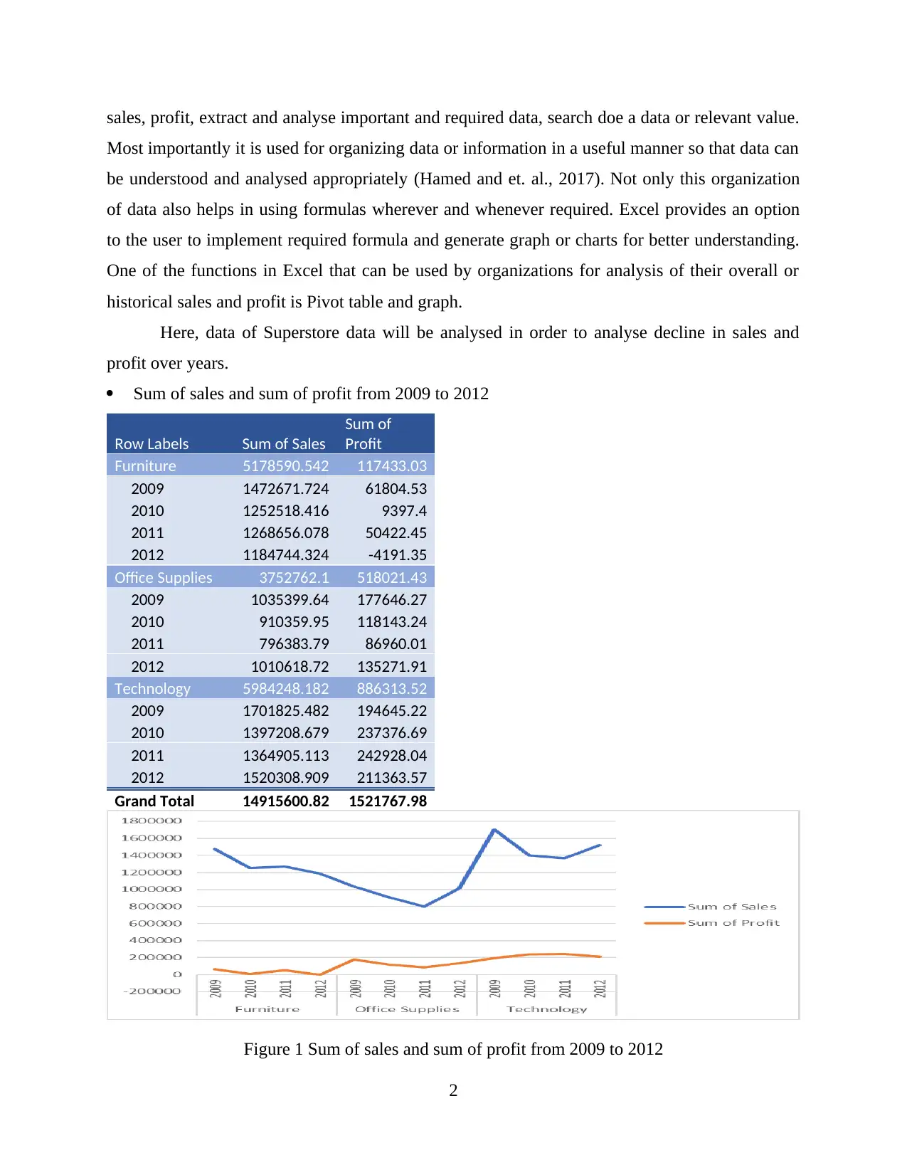
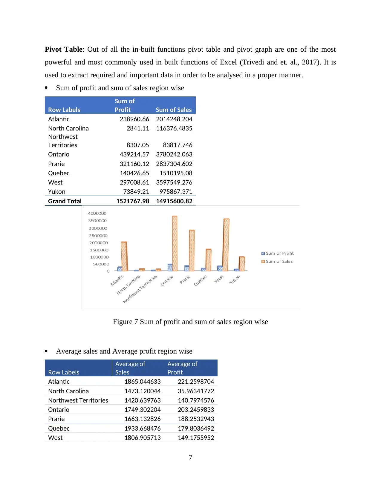
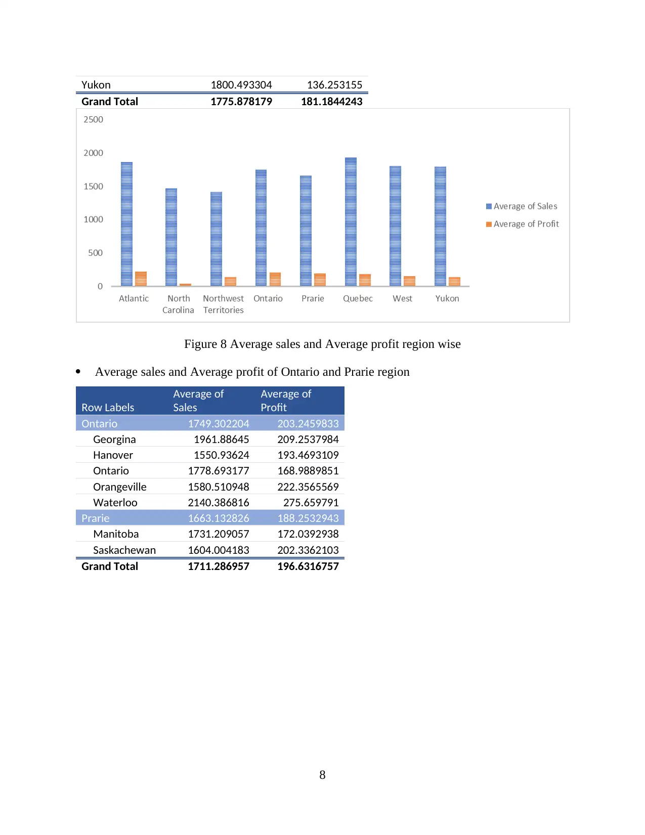
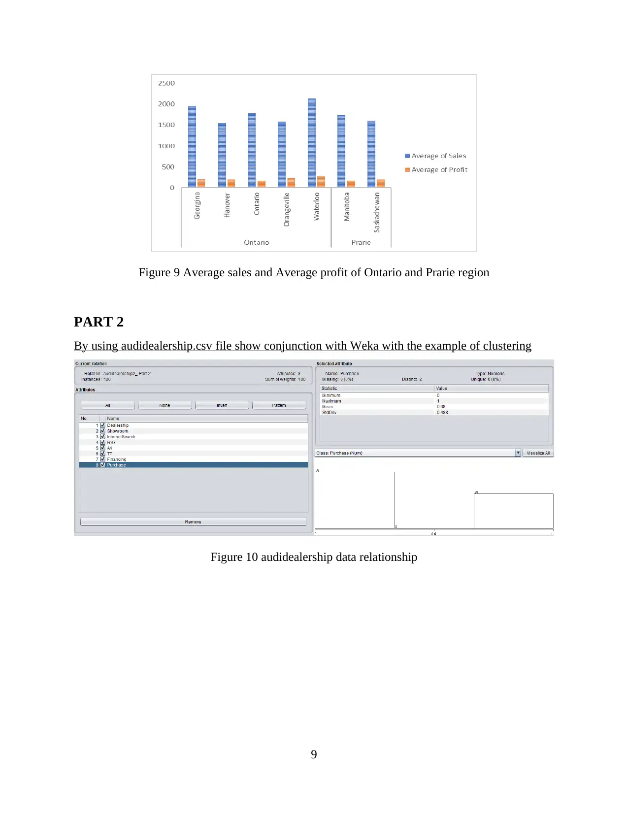
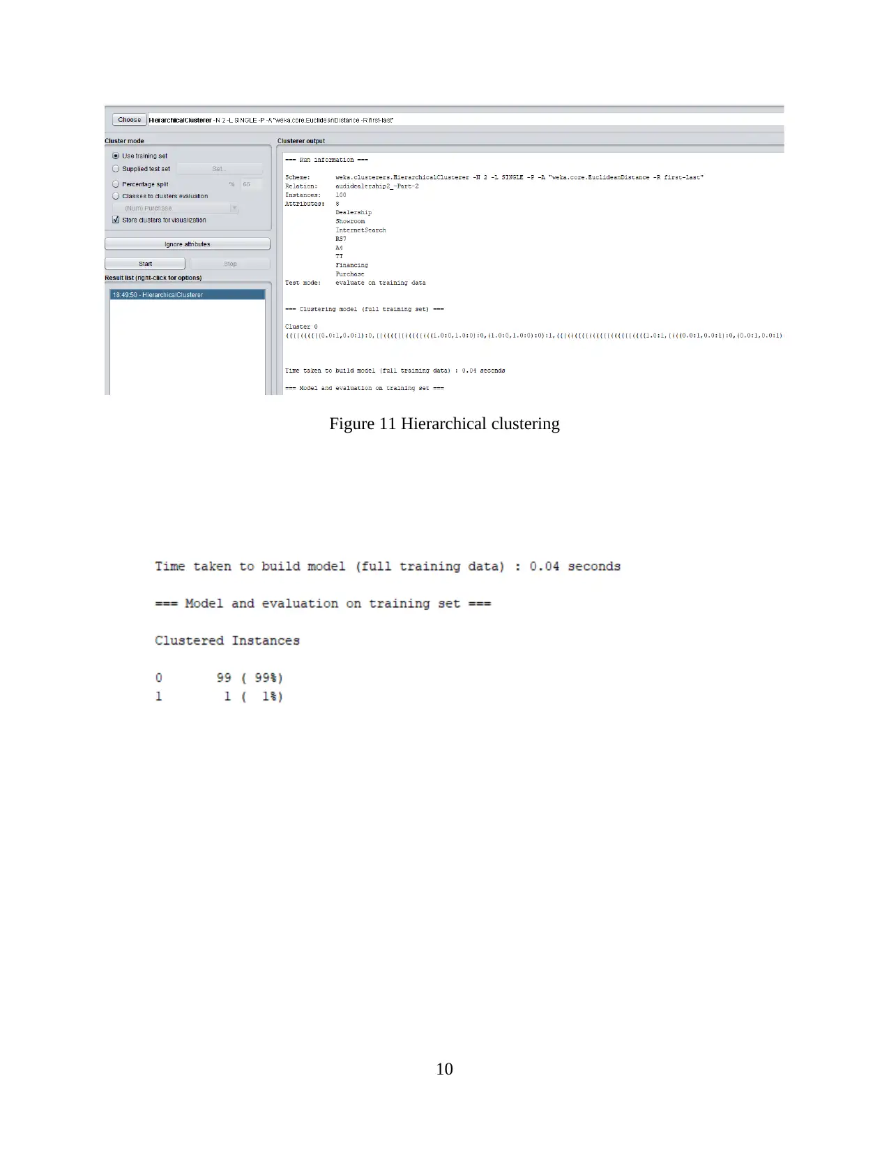
This report provides a comprehensive analysis of data handling and business intelligence, focusing on the analysis of superstore and Audi dealership datasets. The first part of the report utilizes Excel to analyze profit and sales trends over several years, demonstrating the use of pivot tables, graphs, and charts for data visualization and interpretation. The analysis includes the sum of sales and profit, as well as average sales and profit for different product categories. The second part of the report explores data mining techniques using the Weka tool, with a focus on clustering analysis applied to the Audi dealership data. The report also explains commonly used data mining methods such as association and classification, providing real-time examples, and concludes with a comparison of the advantages and disadvantages of Weka. The report offers a detailed overview of data handling processes, data analysis tools, and data mining methods relevant to business intelligence.

DATA HANDLING AND
BUSINESS INTELLIGENCE

TABLE OF CONTENTS
INTRODUCTION...........................................................................................................................1
PART 1............................................................................................................................................1
By using data set of superstores analyse profit and sales over years and analyse it by using
Excel for pre- processing of data, also analyse and visualize the data........................................1
Demonstration of ways in which data can be practically analysed using Excel functions such
as Lookup, Pivot table, graphs and charts...................................................................................6
PART 2............................................................................................................................................9
By using audidealership.csv file show conjunction with Weka with the example of clustering.9
Explanation of commonly used data mining methods that can be used in business. Explain
them with real time example......................................................................................................12
Advantages and disadvantages of Weka....................................................................................13
CONCLUSION..............................................................................................................................13
REREFENCES..............................................................................................................................14

INTRODUCTION
Data handing can be defined as a process through which data can be handled, stores,
disposed off in a secure and safe manner. There are various ways through which data can be
handled. Data handling lies within Business Intelligence as it helps an organization to manage,
store and analyse their data in order to reach to a conclusion. Business Intelligence can be
defined as a technology driven process which is used for data analysis and presentation of
information or data which can further be used by organizations to take important business
decisions (Tirpude, Karandikar and Welekar, 2020). BI helps in providing historical and current
data to be analysed so that predictive views for the business can be generated. Business
intelligence with data mining helps organizations to take effective and appropriate decisions and
develop future business strategies which not only helps them to achieve their defined goals and
objectives but also helps them to enhance their overall revenue and profitability. However, it can
also be said that data mining is a part of Business intelligence (Bayer and et. al., 2017). Both of
them are fruitful for business in different ways like, data mining helps in analysing patterns
within the data. Data mining helps in resolving any kind of issue where as BI helps in decision
making. The only difference between BI and data mining is that data mining is used for small
data set whereas BI is used for huge data sets. This assignment will lay emphasis on analysis of
data of Audi leadership and Superstore data in order to analyse overall sales and profit of the
organization. This assignment will also help in explaining different kinds of data mining methods
that can be used by organizations and advantages and disadvantages of Weka over Excel.
PART 1
By using data set of superstores analyse profit and sales over years and analyse it by using Excel
for pre- processing of data, also analyse and visualize the data
There are various kinds of tools and technologies that can be used for analysis of a data
set and can be used for extracting and analysing useful and important data in an appropriate
manner (Sasikala, Kalaiselvi and Scholar, 2016). These tools can be used by organizations for
analysing their yearly or quarterly sales or profit so that they can take important decision or
develop strategic plans in order to increase sales and profit. Excel is one of the most commonly
used data mining tools which can be used by organizations for analysis of their historical and
current data so that they can take appropriate decisions. It is one of the most commonly preferred
tools because it has various kinds of inbuilt functions that helps in doing calculations, calculate
1

sales, profit, extract and analyse important and required data, search doe a data or relevant value.
Most importantly it is used for organizing data or information in a useful manner so that data can
be understood and analysed appropriately (Hamed and et. al., 2017). Not only this organization
of data also helps in using formulas wherever and whenever required. Excel provides an option
to the user to implement required formula and generate graph or charts for better understanding.
One of the functions in Excel that can be used by organizations for analysis of their overall or
historical sales and profit is Pivot table and graph.
Here, data of Superstore data will be analysed in order to analyse decline in sales and
profit over years.
 Sum of sales and sum of profit from 2009 to 2012
Row Labels Sum of Sales
Sum of
Profit
Furniture 5178590.542 117433.03
2009 1472671.724 61804.53
2010 1252518.416 9397.4
2011 1268656.078 50422.45
2012 1184744.324 -4191.35
Office Supplies 3752762.1 518021.43
2009 1035399.64 177646.27
2010 910359.95 118143.24
2011 796383.79 86960.01
2012 1010618.72 135271.91
Technology 5984248.182 886313.52
2009 1701825.482 194645.22
2010 1397208.679 237376.69
2011 1364905.113 242928.04
2012 1520308.909 211363.57
Grand Total 14915600.82 1521767.98
Figure 1 Sum of sales and sum of profit from 2009 to 2012
2

Figure 2 Sum of sales
Figure 3 Sum of profit
Data Interpretation: All the three graphs above clearly explain decline in sales and profit over
years. First graphs explain both sum of sales over years and sum of profit over years in one graph
so that comparison between both of them can be done. Other two graphs explain sum of sales
and profit individually. From all the threw graphs it has been interpreted that highest sales was
seen in 2009 in Technology department and highest profit was seen in year 2011 in Technology
department.
 Average sales and profit of Technology over years
Row Labels
Average of
Sales
Average of
Profit
Technology 2897.941008 429.2075157
2009 3145.703293 359.7878373
2010 2631.278114 447.037081
2011 2916.463917 519.0770085
2012 2895.826493 402.5972762
Grand Total 2897.941008 429.2075157
3

Figure 4 Average sales and profit of Technology
Data Interpretation: From the above graph it can be clearly interpreted that average sales of
Technology was lowest in 2010 and average profit of technology was lowest in 2009.
 Average sales and profit of Furniture over years
Row Labels
Average of
Sales
Average of
Profit
Furniture 3003.82282 68.11660673
2009 3287.21367 137.9565402
2010 2846.632764 21.35772727
2011 3035.062388 120.6278708
2012 2834.316565 -10.02715311
Grand Total 3003.82282 68.11660673
4

Figure 5 Average sales and profit of Furniture
Data Interpretation: From the above graph it can be interpreted that Average sales of furniture
was highest in 2009 and lowest in 2010 whereas it cannot be determined properly for Average
profit but from the table it can be interpreted that average profit of furniture was highest in 2009
and lowest in 2012.
 Average sales and profit of office Supplies over years
Row Labels
Average of
Sales
Average of
Profit
Office Supplies 814.0481779 112.3690738
2009 885.7139778 151.9643028
2010 778.0854274 100.9771282
2011 716.172473 78.20144784
2012 871.9747368 116.7143313
Grand Total 814.0481779 112.3690738
Figure 6 Average sales and profit of office Supplies
5

Data Interpretation: From the above graph it can be interpreted that average sales of Office
supplies were highest in 2012 and lowest in 2012 whereas average profit of Office supplies was
highest in 2009 and lowest in 2011.
Demonstration of ways in which data can be practically analysed using Excel functions such as
Lookup, Pivot table, graphs and charts
There are various kinds of in-built function present in Excel. Out of all of those lookup
and Pivot table are most commonly used in-built functions of excel.
Lookup Function: This function has been categorised in Excel under Lookup and
Reference functions. This function helps in performing rough match lookup either in one row or
in one column (Massaro and et. al., 2019). It is basically used for selecting values from a defined
range. It is mostly used in financial calculations in which comparison of two rows or column is
required to be done, for this, lookup function can be used. It is basically designed to handle
simplest case of horizontal and vertical look up as well. This formula is basically applied to the
data which is assembled in a particular order. It is basically used for a large amount of data and
in order to find out value of an appropriate data from a huge set of data. The basic syntax used
for lookup function for searching a data is
=LOOKUP (value, loopup_range, [result_range])
For example:
If user wants to find average sales valie in 2011 from the below data then lookup finction can be
used
Row Labels
Average of
Sales
Average of
Profit
Furniture 3003.82282 68.11660673
2009 3287.21367 137.9565402
2010 2846.632764 21.35772727
2011 3035.062388 120.6278708
2012 2834.316565 -10.02715311
=LOOKUP(A5,A3:A6,B3:B6)
3035.062388
6

Pivot Table: Out of all the in-built functions pivot table and pivot graph are one of the most
powerful and most commonly used in built functions of Excel (Trivedi and et. al., 2017). It is
used to extract required and important data in order to be analysed in a proper manner.
 Sum of profit and sum of sales region wise
Row Labels
Sum of
Profit Sum of Sales
Atlantic 238960.66 2014248.204
North Carolina 2841.11 116376.4835
Northwest
Territories 8307.05 83817.746
Ontario 439214.57 3780242.063
Prarie 321160.12 2837304.602
Quebec 140426.65 1510195.08
West 297008.61 3597549.276
Yukon 73849.21 975867.371
Grand Total 1521767.98 14915600.82
Figure 7 Sum of profit and sum of sales region wise
 Average sales and Average profit region wise
Row Labels
Average of
Sales
Average of
Profit
Atlantic 1865.044633 221.2598704
North Carolina 1473.120044 35.96341772
Northwest Territories 1420.639763 140.7974576
Ontario 1749.302204 203.2459833
Prarie 1663.132826 188.2532943
Quebec 1933.668476 179.8036492
West 1806.905713 149.1755952
7

Yukon 1800.493304 136.253155
Grand Total 1775.878179 181.1844243
Figure 8 Average sales and Average profit region wise
 Average sales and Average profit of Ontario and Prarie region
Row Labels
Average of
Sales
Average of
Profit
Ontario 1749.302204 203.2459833
Georgina 1961.88645 209.2537984
Hanover 1550.93624 193.4693109
Ontario 1778.693177 168.9889851
Orangeville 1580.510948 222.3565569
Waterloo 2140.386816 275.659791
Prarie 1663.132826 188.2532943
Manitoba 1731.209057 172.0392938
Saskachewan 1604.004183 202.3362103
Grand Total 1711.286957 196.6316757
8

Figure 9 Average sales and Average profit of Ontario and Prarie region
PART 2
By using audidealership.csv file show conjunction with Weka with the example of clustering
Figure 10 audidealership data relationship
9

Figure 11 Hierarchical clustering
10