Data Analysis and Forecasting: Electricity Bill Prediction Report

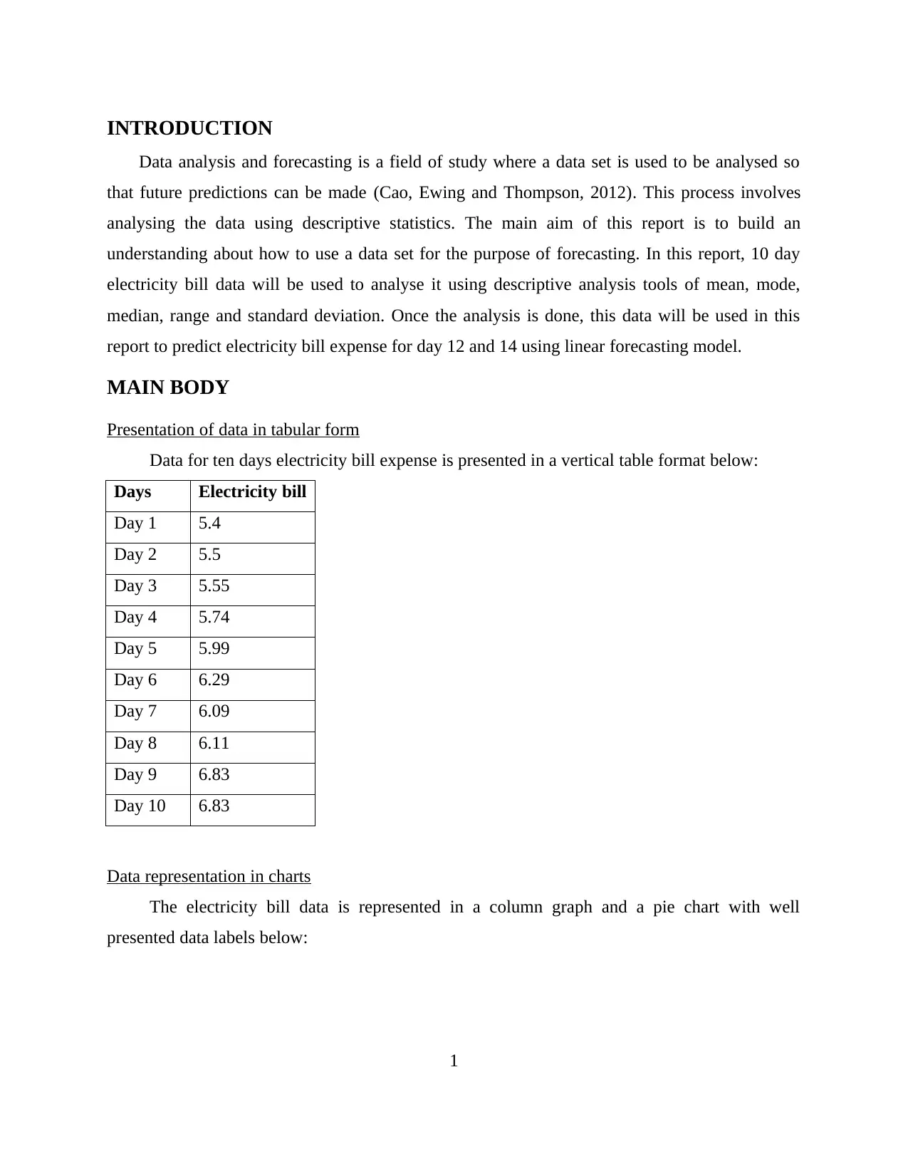
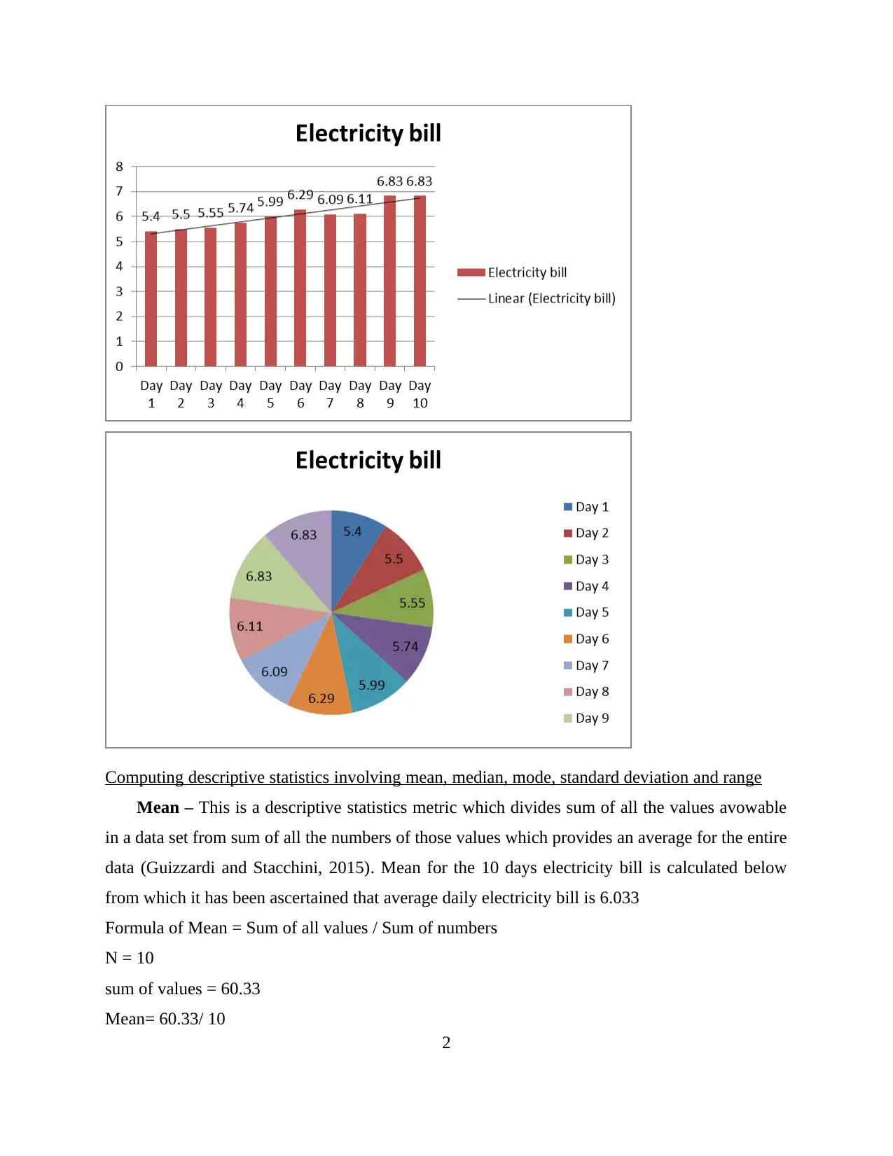
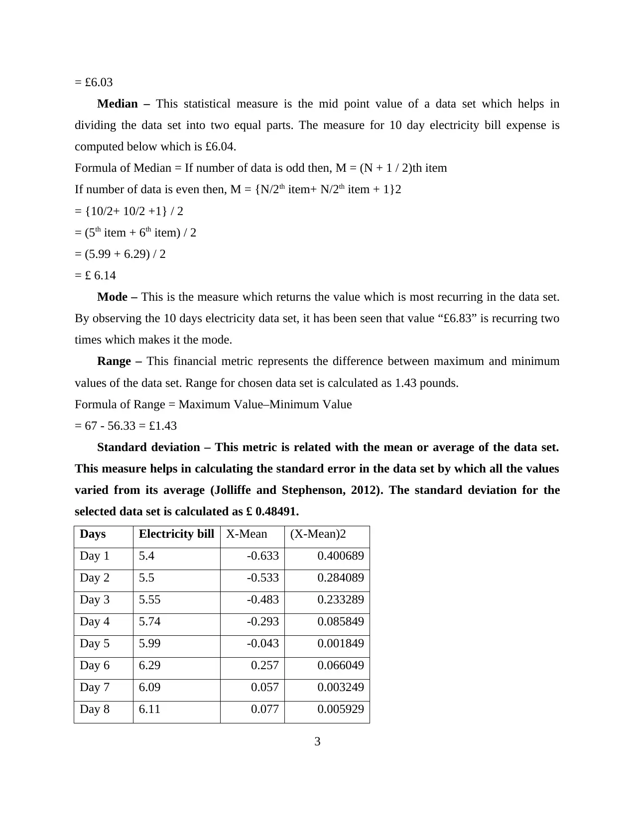
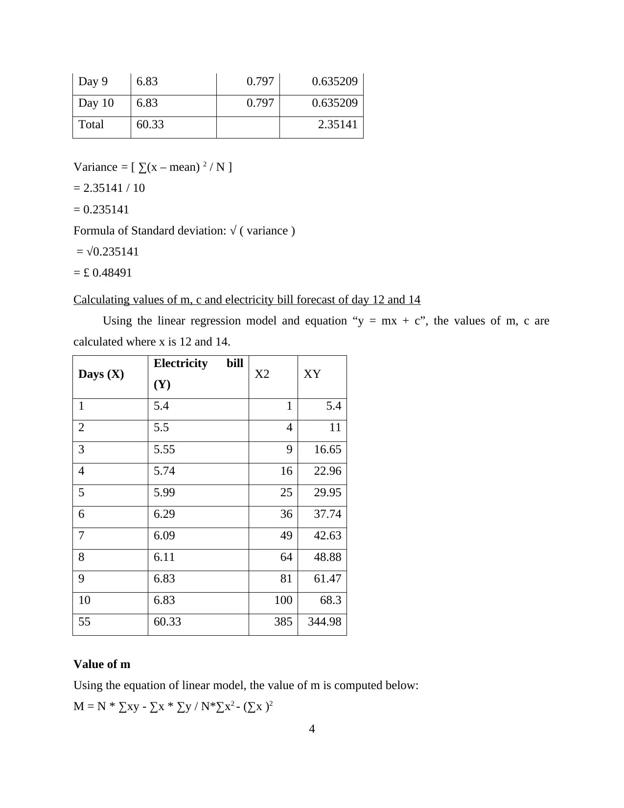
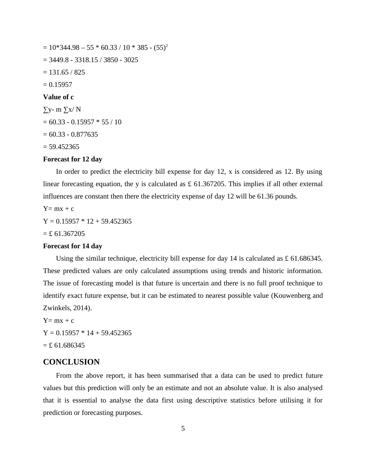
This report focuses on data analysis and forecasting, utilizing a 10-day electricity bill dataset to demonstrate the process of making future predictions. The analysis begins with a presentation of the data in both tabular and chart formats, followed by the computation of descriptive statistics, including mean, median, mode, range, and standard deviation. These statistical measures provide insights into the dataset's characteristics. The report then employs a linear regression model to calculate the values of 'm' and 'c', enabling the forecasting of electricity bill expenses for days 12 and 14. The report concludes by emphasizing that while data can be used for predictive purposes, the forecasts are estimates, and the initial analysis using descriptive statistics is crucial before employing the data for forecasting. References to relevant books and journals are also provided, supporting the methodologies and concepts discussed within the report.

Data Analysis and
Forecasting

Contents
INTRODUCTION...........................................................................................................................1
MAIN BODY..................................................................................................................................1
Presentation of data in tabular form.............................................................................................1
Data representation in charts.......................................................................................................1
Computing descriptive statistics involving mean, median, mode, standard deviation and range
.....................................................................................................................................................2
Calculating values of m, c and electricity bill forecast of day 12 and 14....................................4
CONCLUSION................................................................................................................................5
REFERENCES................................................................................................................................6

INTRODUCTION
Data analysis and forecasting is a field of study where a data set is used to be analysed so
that future predictions can be made (Cao, Ewing and Thompson, 2012). This process involves
analysing the data using descriptive statistics. The main aim of this report is to build an
understanding about how to use a data set for the purpose of forecasting. In this report, 10 day
electricity bill data will be used to analyse it using descriptive analysis tools of mean, mode,
median, range and standard deviation. Once the analysis is done, this data will be used in this
report to predict electricity bill expense for day 12 and 14 using linear forecasting model.
MAIN BODY
Presentation of data in tabular form
Data for ten days electricity bill expense is presented in a vertical table format below:
Days Electricity bill
Day 1 5.4
Day 2 5.5
Day 3 5.55
Day 4 5.74
Day 5 5.99
Day 6 6.29
Day 7 6.09
Day 8 6.11
Day 9 6.83
Day 10 6.83
Data representation in charts
The electricity bill data is represented in a column graph and a pie chart with well
presented data labels below:
1

Computing descriptive statistics involving mean, median, mode, standard deviation and range
Mean – This is a descriptive statistics metric which divides sum of all the values avowable
in a data set from sum of all the numbers of those values which provides an average for the entire
data (Guizzardi and Stacchini, 2015). Mean for the 10 days electricity bill is calculated below
from which it has been ascertained that average daily electricity bill is 6.033
Formula of Mean = Sum of all values / Sum of numbers
N = 10
sum of values = 60.33
Mean= 60.33/ 10
2

= £6.03
Median – This statistical measure is the mid point value of a data set which helps in
dividing the data set into two equal parts. The measure for 10 day electricity bill expense is
computed below which is £6.04.
Formula of Median = If number of data is odd then, M = (N + 1 / 2)th item
If number of data is even then, M = {N/2th item+ N/2th item + 1}2
= {10/2+ 10/2 +1} / 2
= (5th item + 6th item) / 2
= (5.99 + 6.29) / 2
= £ 6.14
Mode – This is the measure which returns the value which is most recurring in the data set.
By observing the 10 days electricity data set, it has been seen that value “£6.83” is recurring two
times which makes it the mode.
Range – This financial metric represents the difference between maximum and minimum
values of the data set. Range for chosen data set is calculated as 1.43 pounds.
Formula of Range = Maximum Value–Minimum Value
= 67 - 56.33 = £1.43
Standard deviation – This metric is related with the mean or average of the data set.
This measure helps in calculating the standard error in the data set by which all the values
varied from its average (Jolliffe and Stephenson, 2012). The standard deviation for the
selected data set is calculated as £ 0.48491.
Days Electricity bill X-Mean (X-Mean)2
Day 1 5.4 -0.633 0.400689
Day 2 5.5 -0.533 0.284089
Day 3 5.55 -0.483 0.233289
Day 4 5.74 -0.293 0.085849
Day 5 5.99 -0.043 0.001849
Day 6 6.29 0.257 0.066049
Day 7 6.09 0.057 0.003249
Day 8 6.11 0.077 0.005929
3

Day 9 6.83 0.797 0.635209
Day 10 6.83 0.797 0.635209
Total 60.33 2.35141
Variance = [ ∑(x – mean) 2 / N ]
= 2.35141 / 10
= 0.235141
Formula of Standard deviation: √ ( variance )
= √0.235141
= £ 0.48491
Calculating values of m, c and electricity bill forecast of day 12 and 14
Using the linear regression model and equation “y = mx + c”, the values of m, c are
calculated where x is 12 and 14.
Days (X) Electricity bill
(Y) X2 XY
1 5.4 1 5.4
2 5.5 4 11
3 5.55 9 16.65
4 5.74 16 22.96
5 5.99 25 29.95
6 6.29 36 37.74
7 6.09 49 42.63
8 6.11 64 48.88
9 6.83 81 61.47
10 6.83 100 68.3
55 60.33 385 344.98
Value of m
Using the equation of linear model, the value of m is computed below:
M = N * ∑xy - ∑x * ∑y / N*∑x2 - (∑x )2
4

= 10*344.98 – 55 * 60.33 / 10 * 385 - (55)2
= 3449.8 - 3318.15 / 3850 - 3025
= 131.65 / 825
= 0.15957
Value of c
∑y- m ∑x/ N
= 60.33 - 0.15957 * 55 / 10
= 60.33 - 0.877635
= 59.452365
Forecast for 12 day
In order to predict the electricity bill expense for day 12, x is considered as 12. By using
linear forecasting equation, the y is calculated as £ 61.367205. This implies if all other external
influences are constant then there the electricity expense of day 12 will be 61.36 pounds.
Y= mx + c
Y = 0.15957 * 12 + 59.452365
= £ 61.367205
Forecast for 14 day
Using the similar technique, electricity bill expense for day 14 is calculated as £ 61.686345.
These predicted values are only calculated assumptions using trends and historic information.
The issue of forecasting model is that future is uncertain and there is no full proof technique to
identify exact future expense, but it can be estimated to nearest possible value (Kouwenberg and
Zwinkels, 2014).
Y= mx + c
Y = 0.15957 * 14 + 59.452365
= £ 61.686345
CONCLUSION
From the above report, it has been summarised that a data can be used to predict future
values but this prediction will only be an estimate and not an absolute value. It is also analysed
that it is essential to analyse the data first using descriptive statistics before utilising it for
prediction or forecasting purposes.
5

REFERENCES
Books and Journals
Cao, Q., Ewing, B.T. and Thompson, M.A., 2012. Forecasting wind speed with recurrent neural
networks. European Journal of Operational Research. 221(1). pp.148-154.
Guizzardi, A. and Stacchini, A., 2015. Real-time forecasting regional tourism with business
sentiment surveys. Tourism Management. 47. pp.213-223.
Jolliffe, I.T. and Stephenson, D.B. eds., 2012. Forecast verification: a practitioner's guide in
atmospheric science. John Wiley & Sons.
Kouwenberg, R. and Zwinkels, R., 2014. Forecasting the US housing market. International
Journal of Forecasting. 30(3). pp.415-425.
6