BUS105 Computing Assignment: Data Analysis and Financial Concepts

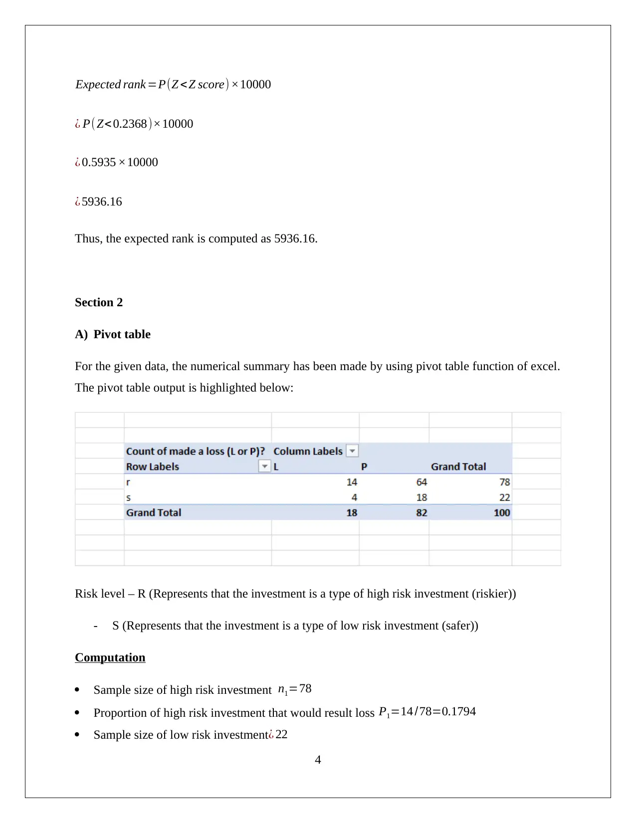
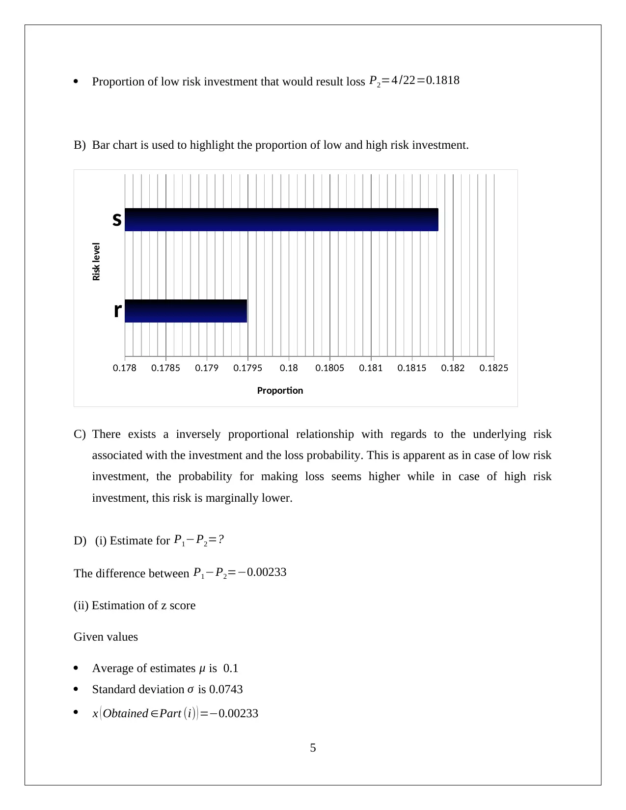
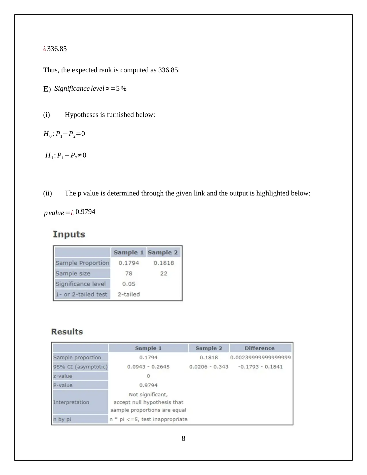
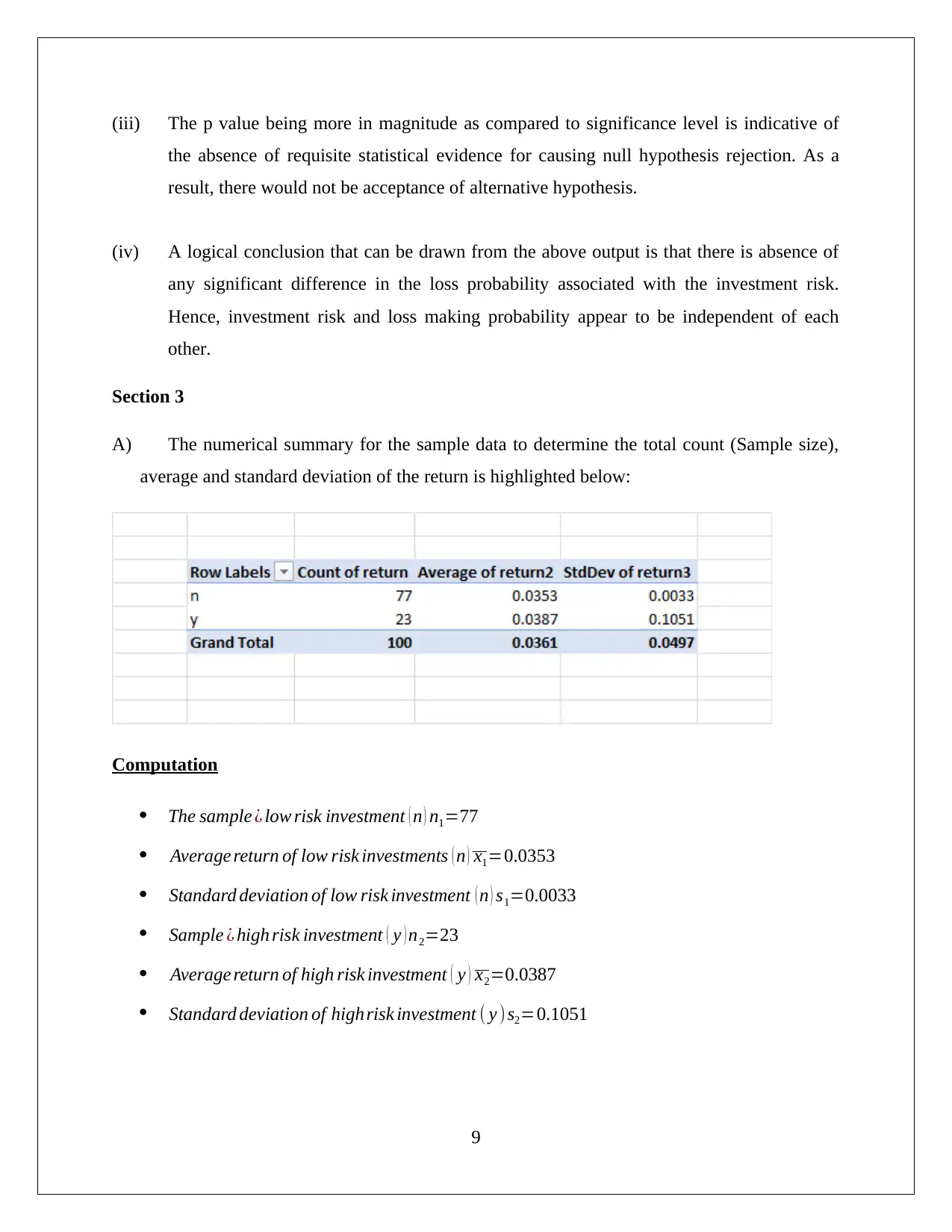
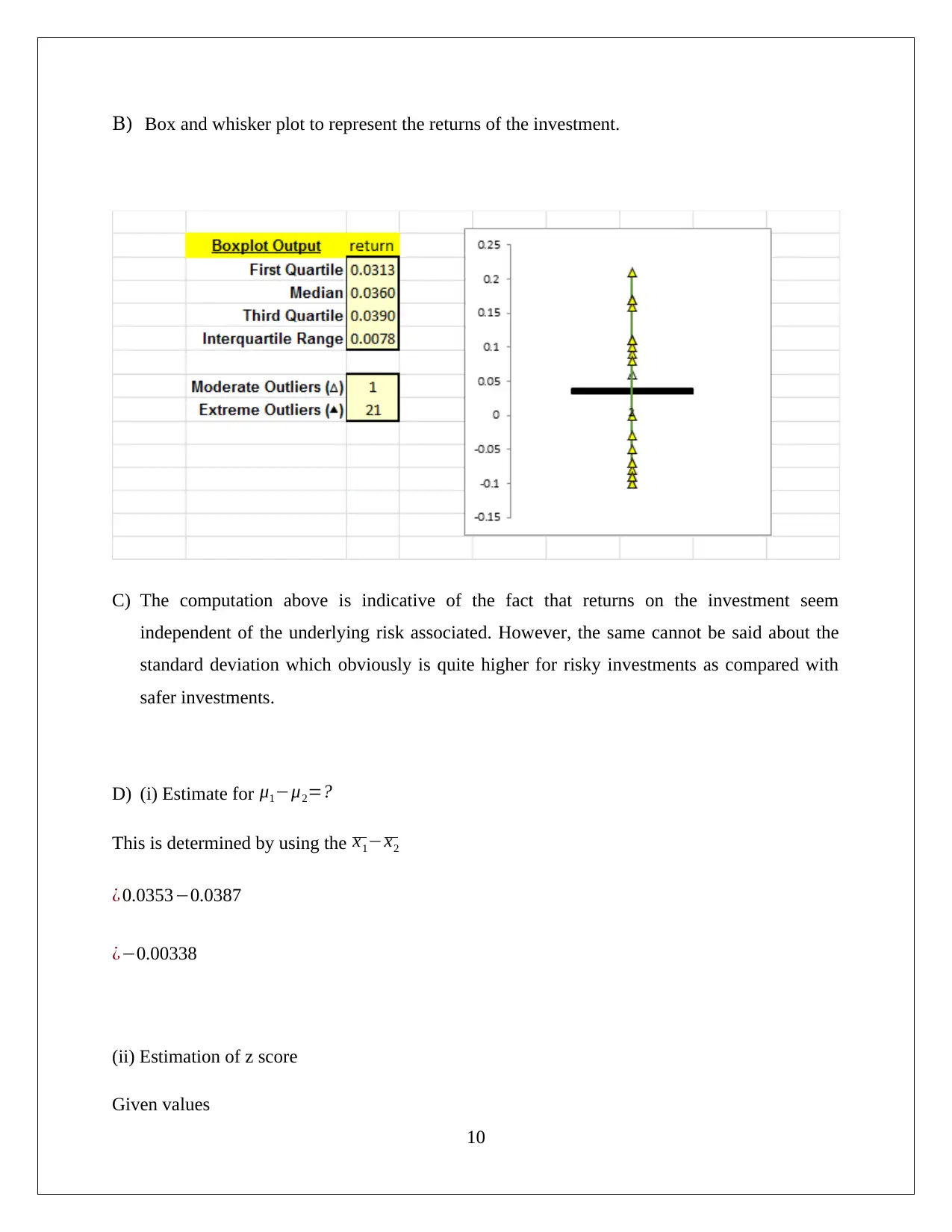
This computing assignment, submitted by Azaz Mahmood for BUS105, demonstrates data analysis and statistical techniques across several sections. Section 1 focuses on scatter plots and regression analysis, exploring the relationship between income and annual contribution. Section 2 uses pivot tables to summarize data on investment risk and loss probability, calculating z-scores and p-values to test hypotheses. Section 3 extends this analysis to investment returns. Section 4 investigates confidence intervals for proportions related to changes. Section 5 uses pivot tables to summarize the relationship between gender and average monthly spending. Finally, Section 6 discusses the application of mean and standard deviation in financial contexts, particularly in portfolio formation, emphasizing the importance of risk and return analysis for investment decisions. The assignment utilizes various statistical tools and concepts to analyze different datasets and draw meaningful conclusions.

Bus105 Computing Assignment
Name: Azaz Mahmood
Student Number: 11600096
Allocated Sample: 9
25-Sep-17

Section 1
Relevant data
A) For the above two variables the scatter plot is highlighted below:
Dependent variable is taken as annual contribution and independent variable is taken as income.
Comment on the relationship: It can be seen from the scatter plot that moderate to strong
relationship is existing between the independent and dependent variable. Further, the positive
1

slope indicates that income and annual contribution is having positive linear relationship, which
means as the income increases the annual contribution would also be increased.
B) From the scatter plot the regression line can be obtained and is shown below:
Y =0.1616 x −4822.6
Representation:
X= dependent variable = Income ($)
Y = independent variable = Annual contribution ($)
The next task is to determine the annual contribution for the income amount (x) of $200,000.
Now,
Y =(0.1616 ×200,000)−4822.6
Y =32320−4822.6
Y =$ 27497.4
Hence, the computed value of annual contribution for income amount $200,000 is $ 27 , 497.4 .
C) Estimation of z score
Given values
 Average of estimates μ is $27,000
 Standard deviation σ is $2,100
 x ( Obtained∈Part B ) =$ 27497.4
Formula for z score
z= ( x −μ
σ )
2

z= (27497.4−27000
2100 )
z score=0.2368
Hence, the value of z score is computed as 0.2368.
D) By using the given link, the value of P(Z<Z score) i.e. P ( Z <0.2368 ) has been computed and
is shown below:
E) List of estimates = 10,000
Hence,
3

Expected rank =P(Z <Z score) ×10000
¿ P(Z< 0.2368)×10000
¿ 0.5935 ×10000
¿ 5936.16
Thus, the expected rank is computed as 5936.16.
Section 2
A) Pivot table
For the given data, the numerical summary has been made by using pivot table function of excel.
The pivot table output is highlighted below:
Risk level – R (Represents that the investment is a type of high risk investment (riskier))
- S (Represents that the investment is a type of low risk investment (safer))
Computation
 Sample size of high risk investment n1=78
 Proportion of high risk investment that would result loss P1=14 /78=0.1794
 Sample size of low risk investment ¿ 22
4

 Proportion of low risk investment that would result loss P2=4 /22=0.1818
B) Bar chart is used to highlight the proportion of low and high risk investment.
r
s
0.178 0.1785 0.179 0.1795 0.18 0.1805 0.181 0.1815 0.182 0.1825
Proportion
Risk level
C) There exists a inversely proportional relationship with regards to the underlying risk
associated with the investment and the loss probability. This is apparent as in case of low risk
investment, the probability for making loss seems higher while in case of high risk
investment, this risk is marginally lower.
D) (i) Estimate for P1−P2=?
The difference between P1−P2=−0.00233
(ii) Estimation of z score
Given values
 Average of estimates μ is 0.1
 Standard deviation σ is 0.0743
 x ( Obtained ∈Part (i) ) =−0.00233
5

Formula for z score
z= ( x −μ
σ )
z= ( −0.00233−0.1
0.0743 )
z score=−1.377
Hence, the value of z score is computed as -1.377.
(iii) By using the given link, the value of P(Z<Z score) i.e. P ( Z <−1.377 ) has been computed
and is shown below:
6

(iv) List of estimates = 4,000
Hence,
Expected rank =P(Z <Z score) ×4000
¿ P(Z<−1.377)× 4000
¿ 0.0842 ×4000
7

¿ 336.85
Thus, the expected rank is computed as 336.85.
E) Significance level ∝=5 %
(i) Hypotheses is furnished below:
H0 : P1−P2=0
H1 : P1 −P2 ≠ 0
(ii) The p value is determined through the given link and the output is highlighted below:
p value=¿ 0.9794
8

(iii) The p value being more in magnitude as compared to significance level is indicative of
the absence of requisite statistical evidence for causing null hypothesis rejection. As a
result, there would not be acceptance of alternative hypothesis.
(iv) A logical conclusion that can be drawn from the above output is that there is absence of
any significant difference in the loss probability associated with the investment risk.
Hence, investment risk and loss making probability appear to be independent of each
other.
Section 3
A) The numerical summary for the sample data to determine the total count (Sample size),
average and standard deviation of the return is highlighted below:
Computation
 The sample ¿ low risk investment ( n ) n1=77
 Average return of low risk investments ( n ) x1=0.0353
 Standard deviation of low risk investment ( n ) s1=0.0033
 Sample ¿ high risk investment ( y ) n2=23
 Average return of high risk investment ( y ) x2=0.0387
 Standard deviation of highrisk investment ( y )s2=0.1051
9

B) Box and whisker plot to represent the returns of the investment.
C) The computation above is indicative of the fact that returns on the investment seem
independent of the underlying risk associated. However, the same cannot be said about the
standard deviation which obviously is quite higher for risky investments as compared with
safer investments.
D) (i) Estimate for μ1−μ2=?
This is determined by using the x1−x2
¿ 0.0353−0.0387
¿−0.00338
(ii) Estimation of z score
Given values
10

 Average of estimates μ is -0.0256
 Standard deviation σ is 0.0173
 x ( Obtained ∈Part (i) ) =−0.00338
Formula for z score
z= ( x −μ
σ )
z= ( −0.00338−−0.0256
0.0173 )
z score=−1.6753
Hence, the value of z score is computed as −1.6753
(iii) By using the given link, the value of P(Z<Z score) i.e. P ( Z <−1.6753 ) has been
computed and is shown below:
11