Data Analysis Assignment: Bill Payment Analysis and Prediction

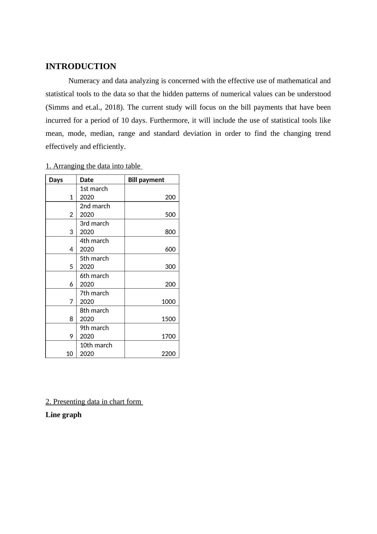
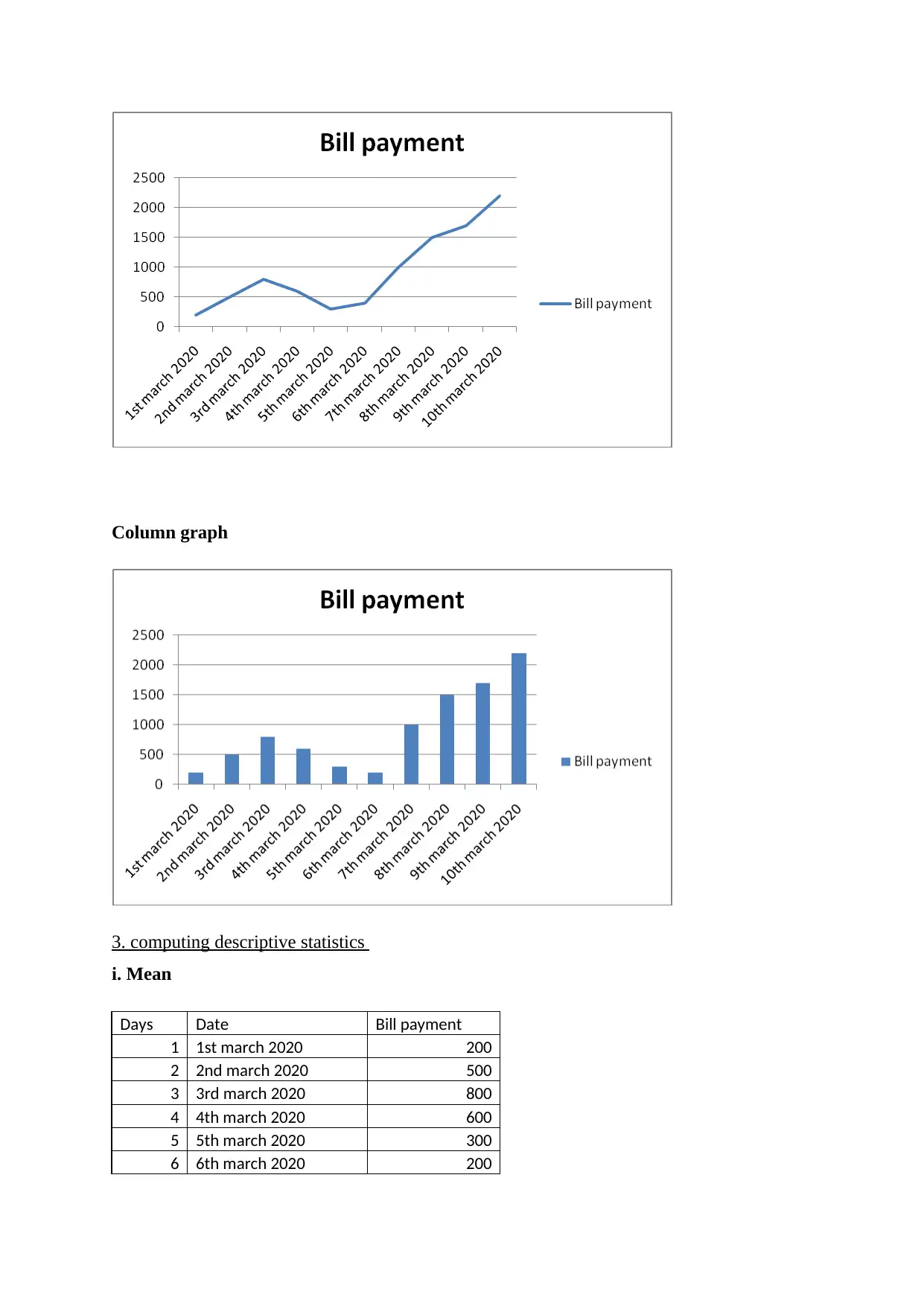
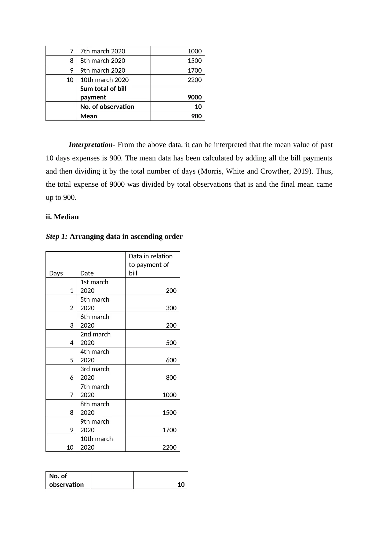
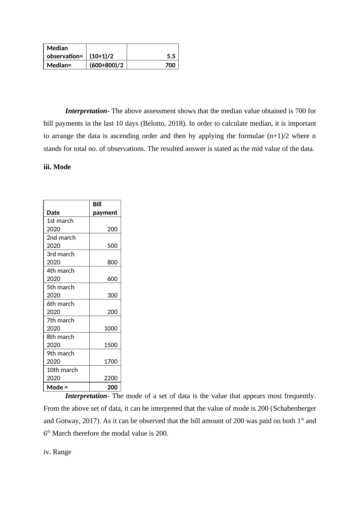
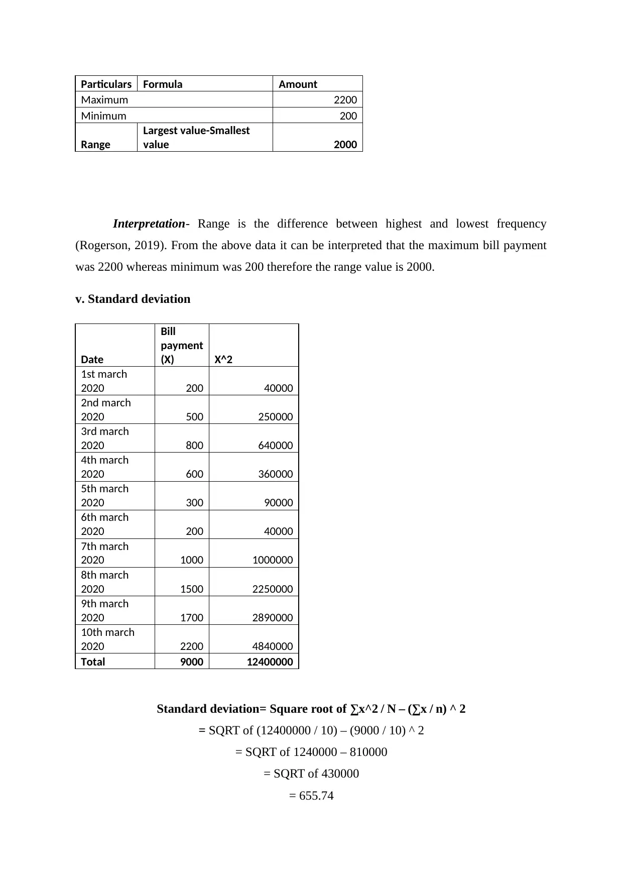
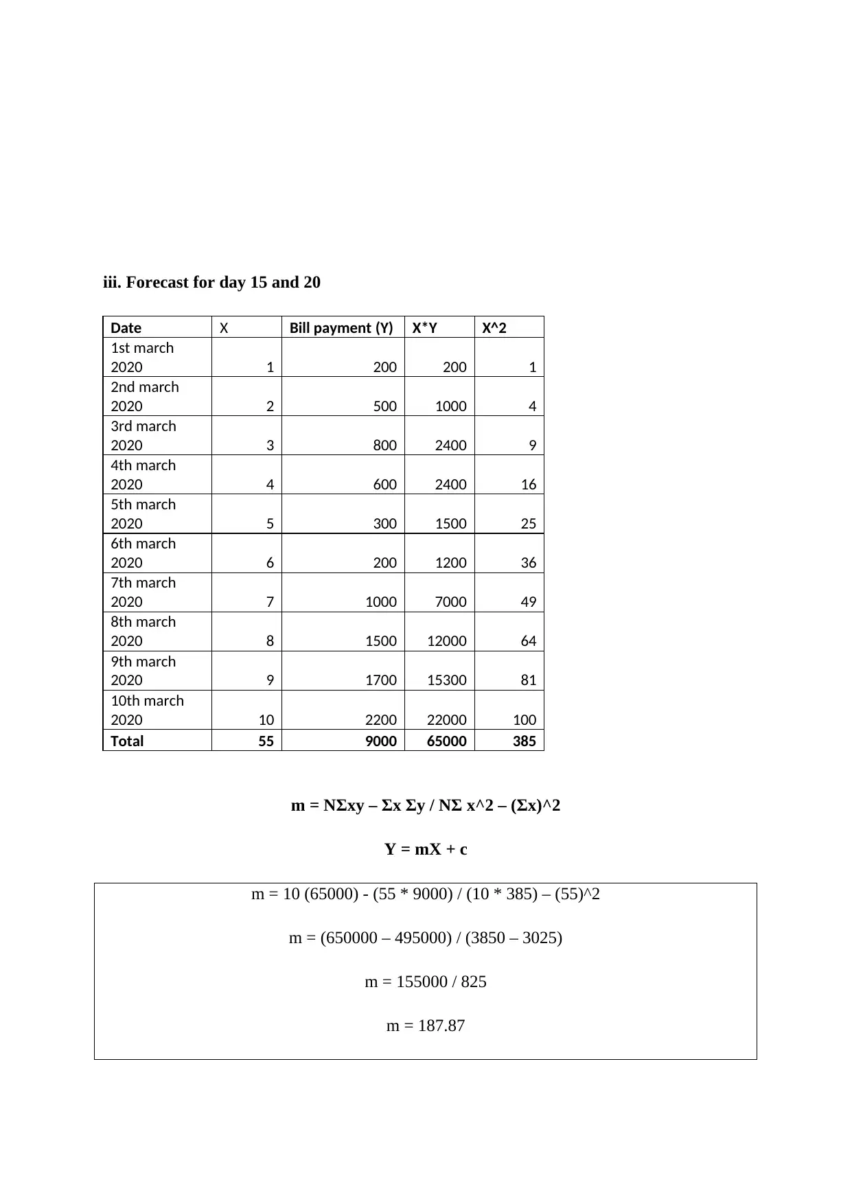
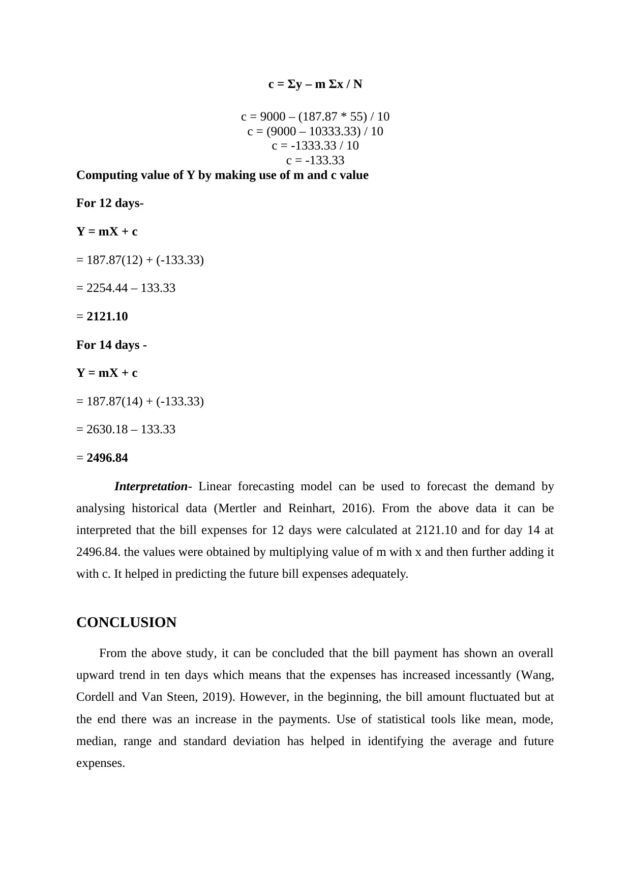
This data analysis assignment examines bill payment data collected over a ten-day period. The analysis begins by organizing the data into tables and presenting it visually using line and column graphs. Descriptive statistics, including mean, median, mode, range, and standard deviation, are calculated to identify trends and patterns in the payment amounts. Furthermore, a linear forecasting model is employed to predict bill payments for the 15th and 20th days, demonstrating the practical application of these statistical tools. The assignment concludes with an interpretation of the findings, highlighting the increasing trend in bill payments and the utility of statistical methods for understanding and predicting future expenses. The student used references from various books and journals to support the analysis.

Data Analysis

INTRODUCTION......................................................................................................................3
1. Arranging the data into table..............................................................................................3
2. Presenting data in chart form.............................................................................................3
3. computing descriptive statistics.........................................................................................4
4. Using the linear forecasting model for predicting the value for 15 and 20 day.................8
CONCLUSION........................................................................................................................10
REFERENCES.........................................................................................................................11

INTRODUCTION
Numeracy and data analyzing is concerned with the effective use of mathematical and
statistical tools to the data so that the hidden patterns of numerical values can be understood
(Simms and et.al., 2018). The current study will focus on the bill payments that have been
incurred for a period of 10 days. Furthermore, it will include the use of statistical tools like
mean, mode, median, range and standard deviation in order to find the changing trend
effectively and efficiently.
1. Arranging the data into table
Days Date Bill payment
1
1st march
2020 200
2
2nd march
2020 500
3
3rd march
2020 800
4
4th march
2020 600
5
5th march
2020 300
6
6th march
2020 200
7
7th march
2020 1000
8
8th march
2020 1500
9
9th march
2020 1700
10
10th march
2020 2200
2. Presenting data in chart form
Line graph

Column graph
3. computing descriptive statistics
i. Mean
Days Date Bill payment
1 1st march 2020 200
2 2nd march 2020 500
3 3rd march 2020 800
4 4th march 2020 600
5 5th march 2020 300
6 6th march 2020 200

7 7th march 2020 1000
8 8th march 2020 1500
9 9th march 2020 1700
10 10th march 2020 2200
Sum total of bill
payment 9000
No. of observation 10
Mean 900
Interpretation- From the above data, it can be interpreted that the mean value of past
10 days expenses is 900. The mean data has been calculated by adding all the bill payments
and then dividing it by the total number of days (Morris, White and Crowther, 2019). Thus,
the total expense of 9000 was divided by total observations that is and the final mean came
up to 900.
ii. Median
Step 1: Arranging data in ascending order
Days Date
Data in relation
to payment of
bill
1
1st march
2020 200
2
5th march
2020 300
3
6th march
2020 200
4
2nd march
2020 500
5
4th march
2020 600
6
3rd march
2020 800
7
7th march
2020 1000
8
8th march
2020 1500
9
9th march
2020 1700
10
10th march
2020 2200
No. of
observation 10

Median
observation= (10+1)/2 5.5
Median= (600+800)/2 700
Interpretation- The above assessment shows that the median value obtained is 700 for
bill payments in the last 10 days (Belotto, 2018). In order to calculate median, it is important
to arrange the data is ascending order and then by applying the formulae (n+1)/2 where n
stands for total no. of observations. The resulted answer is stated as the mid value of the data.
iii. Mode
Date
Bill
payment
1st march
2020 200
2nd march
2020 500
3rd march
2020 800
4th march
2020 600
5th march
2020 300
6th march
2020 200
7th march
2020 1000
8th march
2020 1500
9th march
2020 1700
10th march
2020 2200
Mode = 200
Interpretation- The mode of a set of data is the value that appears most frequently.
From the above set of data, it can be interpreted that the value of mode is 200 (Schabenberger
and Gotway, 2017). As it can be observed that the bill amount of 200 was paid on both 1st and
6th March therefore the modal value is 200.
iv. Range

Particulars Formula Amount
Maximum 2200
Minimum 200
Range
Largest value-Smallest
value 2000
Interpretation- Range is the difference between highest and lowest frequency
(Rogerson, 2019). From the above data it can be interpreted that the maximum bill payment
was 2200 whereas minimum was 200 therefore the range value is 2000.
v. Standard deviation
Date
Bill
payment
(X) X^2
1st march
2020 200 40000
2nd march
2020 500 250000
3rd march
2020 800 640000
4th march
2020 600 360000
5th march
2020 300 90000
6th march
2020 200 40000
7th march
2020 1000 1000000
8th march
2020 1500 2250000
9th march
2020 1700 2890000
10th march
2020 2200 4840000
Total 9000 12400000
Standard deviation= Square root of ∑x^2 / N – (∑x / n) ^ 2
= SQRT of (12400000 / 10) – (9000 / 10) ^ 2
= SQRT of 1240000 – 810000
= SQRT of 430000
= 655.74

Interpretation- From the above assessment it can be reflected that the calculated
standard deviation equals to 655.74. The value can be computed by working out the value of
mean and then subtracting it from the square root result (Dorie and et.al., 2019). At last, the
mean of squared differences is worked with square root of difference value.
4. Using the linear forecasting model for predicting the value for 15 and 20 day

iii. Forecast for day 15 and 20
Date X Bill payment (Y) X*Y X^2
1st march
2020 1 200 200 1
2nd march
2020 2 500 1000 4
3rd march
2020 3 800 2400 9
4th march
2020 4 600 2400 16
5th march
2020 5 300 1500 25
6th march
2020 6 200 1200 36
7th march
2020 7 1000 7000 49
8th march
2020 8 1500 12000 64
9th march
2020 9 1700 15300 81
10th march
2020 10 2200 22000 100
Total 55 9000 65000 385
m = NΣxy – Σx Σy / NΣ x^2 – (Σx)^2
Y = mX + c
m = 10 (65000) - (55 * 9000) / (10 * 385) – (55)^2
m = (650000 – 495000) / (3850 – 3025)
m = 155000 / 825
m = 187.87

c = Σy – m Σx / N
c = 9000 – (187.87 * 55) / 10
c = (9000 – 10333.33) / 10
c = -1333.33 / 10
c = -133.33
Computing value of Y by making use of m and c value
For 12 days-
Y = mX + c
= 187.87(12) + (-133.33)
= 2254.44 – 133.33
= 2121.10
For 14 days -
Y = mX + c
= 187.87(14) + (-133.33)
= 2630.18 – 133.33
= 2496.84
Interpretation- Linear forecasting model can be used to forecast the demand by
analysing historical data (Mertler and Reinhart, 2016). From the above data it can be
interpreted that the bill expenses for 12 days were calculated at 2121.10 and for day 14 at
2496.84. the values were obtained by multiplying value of m with x and then further adding it
with c. It helped in predicting the future bill expenses adequately.
CONCLUSION
From the above study, it can be concluded that the bill payment has shown an overall
upward trend in ten days which means that the expenses has increased incessantly (Wang,
Cordell and Van Steen, 2019). However, in the beginning, the bill amount fluctuated but at
the end there was an increase in the payments. Use of statistical tools like mean, mode,
median, range and standard deviation has helped in identifying the average and future
expenses.

REFERENCES
Books and journals
Belotto, M. J., 2018. Data analysis methods for qualitative research: Managing the challenges
of coding, interrater reliability, and thematic analysis. The Qualitative Report. 23(11).
pp.2622-2633.
Dorie, V. and et.al., 2019. Automated versus do-it-yourself methods for causal inference:
Lessons learned from a data analysis competition. Statistical Science. 34(1). pp.43-68.
Mertler, C. A. and Reinhart, R. V., 2016. Advanced and multivariate statistical methods:
Practical application and interpretation. Taylor & Francis.
Morris, T. P., White, I. R. and Crowther, M. J., 2019. Using simulation studies to evaluate
statistical methods. Statistics in medicine, 38(11), pp.2074-2102.
Rogerson, P. A., 2019. Statistical methods for geography: a student’s guide. SAGE
Publications Limited.
Schabenberger, O. and Gotway, C. A., 2017. Statistical methods for spatial data analysis.
CRC press.
Simms, V. and et.al., 2018. Does early home environment influence basic numeracy skills?
The Preparing for Life Study. In Extending the learning from the Prevention and Early
Intervention Initiative (pp. 69-72).
Wang, M. H., Cordell, H. J. and Van Steen, K., 2019, April. Statistical methods for genome-
wide association studies. In Seminars in cancer biology (Vol. 55, pp. 53-60). Academic Press.