Data Analysis & Forecasting Report - Numeracy and Data Analysis BABS

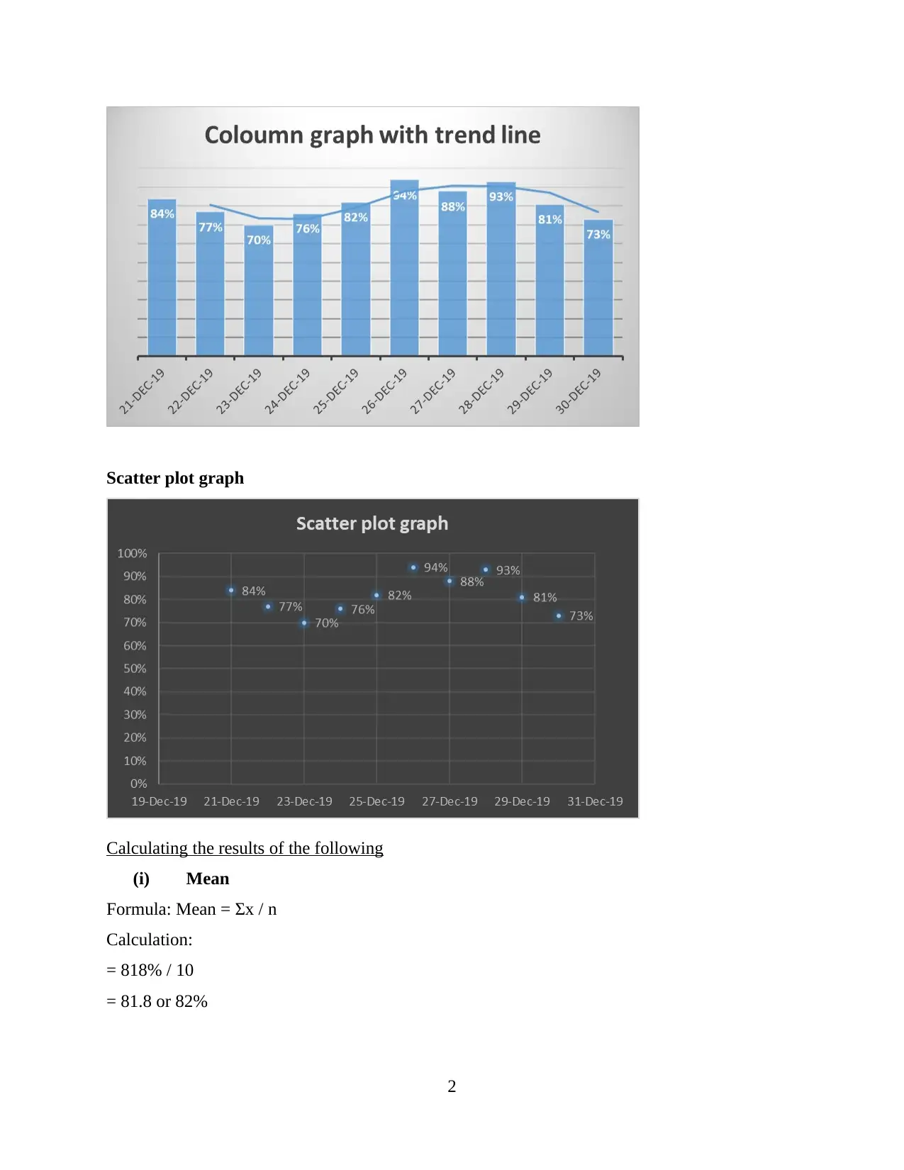
This report presents a data analysis and forecasting exercise using humidity data collected from Birmingham, United Kingdom, over ten consecutive days. The data is presented in tabular format and visualized using column and scatter plot graphs. Descriptive statistics, including mean, median, mode, range, and standard deviation, are calculated to analyze the data's central tendency and dispersion. Furthermore, a linear forecasting model is applied to predict humidity values for the 15th and 20th days, demonstrating the application of forecasting techniques. The report concludes by highlighting the importance of data analysis techniques in transforming raw information into meaningful insights for decision-making.

Individual project

Contents
INTRODUCTION...........................................................................................................................1
MAIN BODY..................................................................................................................................1
Using table format to present the data set....................................................................................1
Using two types of chart to present the data set..........................................................................1
Calculating the results of the following.......................................................................................2
Using linear forecasting model to calculate the following..........................................................4
CONCLUSION................................................................................................................................6
REFERENCES................................................................................................................................7

INTRODUCTION
Data analysis techniques are the methods of converting the raw information into a
meaningful data which can be used for further purposes. Such techniques are used by
investigators to interpret the data in order to gain useful insights (Wagner-Muns and et.al., 2017).
The present report is developed with the aim to collect humidity percent data of ten consequence
days and then present and analyse it. This report includes humid data of Birmingham, United
Kingdom which is then analysed using descriptive statistics and linear forecasting model.
MAIN BODY
Using table format to present the data set
Date Humidity level
21-Dec-19 84%
22-Dec-19 77%
23-Dec-19 70%
24-Dec-19 76%
25-Dec-19 82%
26-Dec-19 94%
27-Dec-19 88%
28-Dec-19 93%
29-Dec-19 81%
30-Dec-19 73%
The data presented above is gained from Birmingham weather source and the humidity
percentage is recoded at 12:00 Noon for ten days varying from 21 December 2019 to 30
December 2019 (Humidity level in Birmingham, United Kingdom, 2019).
Using two types of chart to present the data set
Column graph with trend line
1

Scatter plot graph
Calculating the results of the following
(i) Mean
Formula: Mean = Σx / n
Calculation:
= 818% / 10
= 81.8 or 82%
2

Mean is the statistical average which is determined by dividing the total number of
frequencies to sum of the values of all the frequencies (Chang, 2017). In case of humidity data of
Birmingham, the average humidity level for ten days is 82%.
(ii) Median
Formula: Median = (n + 1) / 2
Calculation:
= (10 + 1) / 2
= 5.5 or 6th position
This is a descriptive statistical tool which returns the middle value of the data set. The
entire data set is first arranged in ascending order and then median is ascertained. In this case of
Birmingham humidity data set, the middle value point is 6th and its frequency value is 82%. This
value splits the whole data set of ten days into two equal parts.
(iii) Mode
Mode is the most recurring frequency value of the data set (Pole, West and Harrison, 2018).
In the case of Birmingham, there is no frequency which repeats more than one time due to which
there is no mode in the identified data set. This implies that the humidity level of this region
highly fluctuates and there is no common humidity level which recurs most often.
(iv) Range
Formula: Range = Maximum frequency value – Minimum frequency value
Calculation:
= 94% - 70%
= 24%
Range is the statistical tool which refers to the difference between highest value of the
frequency and lowest value of the frequency. In this case of Birmingham, the range which is
calculated as 24% is the difference between highest value of the frequency that is 94% and
lowest value of the frequency that is 70%.
(v) Standard deviation
Formula: Standard Deviations = √ (variance)
Variance 2 = {∑ (x – mean) / N}2
= {∑ (x2 / N – (mean)2}
Calculation:
3

= (675% / 10) – 82%2
= 67.5% - 67%
= 0.5%
Standard deviation is the standard mean of error which presents how disperse the values
of the data set are. This measure or the case of Birmingham is calculated as 0.5%. This standard
deviation is less than one which means the dispersion rate in the identified humidity data set is
low.
Working notes:
Humidity level (X) X2
84% 71%
77% 59%
70% 49%
76% 58%
82% 67%
94% 88%
88% 77%
93% 86%
81% 66%
73% 53%
Sum of X2 675%
Using linear forecasting model to calculate the following
(i) Value of “m”
Date Day (X) Humidity data (%) (Y) XY X^2
21-Dec-19 1 84% 84% 1
22-Dec-19 2 77% 154% 4
23-Dec-19 3 70% 210% 9
24-Dec-19 4 76% 304% 16
25-Dec-19 5 82% 410% 25
26-Dec-19 6 94% 564% 36
27-Dec-19 7 88% 616% 49
4

28-Dec-19 8 93% 744% 64
29-Dec-19 9 81% 729% 81
30-Dec-19 10 73% 730% 100
Total 55 818% 4545% 385
Particulars Details
m NΣxy – Σx Σy / NΣ x ^ 2 – (Σx) ^ 2
(10 * 4545) - (55 * 818) / (10 * 385) - (55) ^ 2
(45450 - 44990) / (3850 - 3025)
0.55
The value of “m” is calculated above for the purpose of applying linear forecasting model
so that the humidity level of day 15th and day 20th can be ascertained (Xie and et.al., 2016). This
“m” value is calculated using sum of ten days and their humidity level by which a rate of
predictability is computed as 0.55.
(ii) Value of “c”
Particulars Details
c Σy - m Σx / N
(818-(0.55*55))/10
78.77
The value of “c” is also calculated for the purpose of using linear forecasting (Saber and
Alam, 2017). The value of c is computed by using the predictability rate and sum of ten days.
78.77 is determined as c in this case of Birmingham.
(iii) Forecasted humidity value of day 15 and day 20
Forecast of 15th day
y = mx + c
y 0.55 (x) + 78.77
x 15
y 0.55 (15) + 78.77
87.02
Above, the linear forecasting model is used in which equation of y = mx + c is applied.
This equation is used to predict the humidity value of day 15th which is 87.02 or 87%.
5

Forecast of 20th day
y = mx + c
y 0.55 (x) + 78.77
x 20
y 0.55 (20) + 78.77
89.77
From the above numerical analysis, it is observed that the humidity level of 20th day or 9
January is predicted as 89.77 or 90%.
CONCLUSION
After developing the above report, it has been summarised that data analysis techniques
are more of a process which includes the collecting, cleansing, transforming, analysing and then
interpreting the data by which raw information can be used for making decisions. It is also
concluded that linear forecasting model is most appropriate for predicting future values.
6

REFERENCES
Books and Journals
Chang, V., 2017. Towards data analysis for weather cloud computing. Knowledge-Based
Systems. 127. pp.29-45.
Pole, A., West, M. and Harrison, J., 2018. Applied Bayesian forecasting and time series analysis.
Chapman and Hall/CRC.
Saber, A. Y. and Alam, A. R., 2017. Short term load forecasting using multiple linear regression
for big data. In 2017 IEEE Symposium Series on Computational Intelligence (SSCI) (pp.
1-6). IEEE.
Wagner-Muns, I. M. and et.al., 2017. A functional data analysis approach to traffic volume
forecasting. IEEE Transactions on Intelligent Transportation Systems. 19(3). pp.878-888.
Xie, J. and et.al., 2016. Relative humidity for load forecasting models. IEEE Transactions on
Smart Grid. 9(1). pp.191-198.
Online
Humidity level in Birmingham, United Kingdom. 2019. [Online]. Available through:
<https://www.worldweatheronline.com/birmingham-weather-history/west-midlands/
gb.aspx >
7