Data Analytics and Business Intelligence Assignment Solution Report

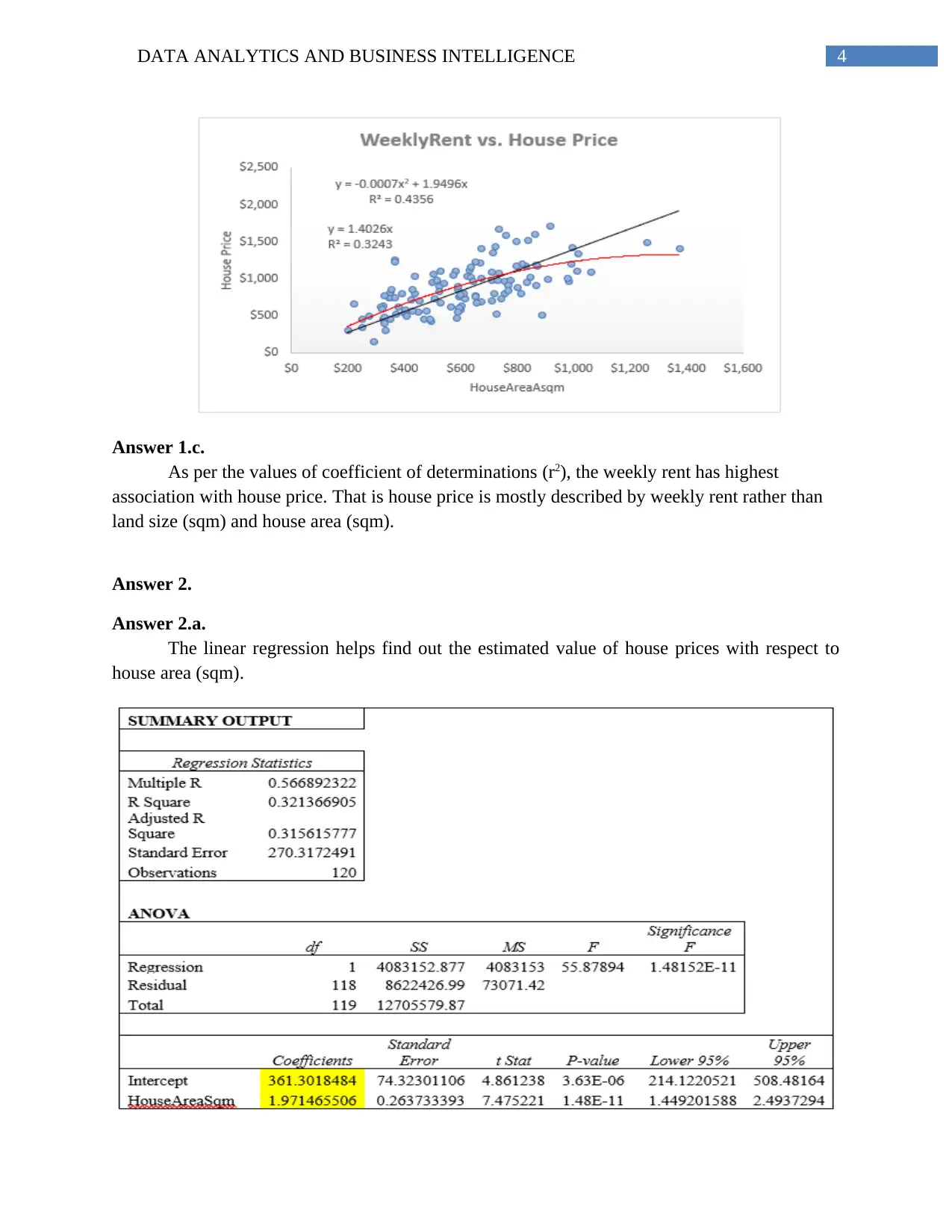
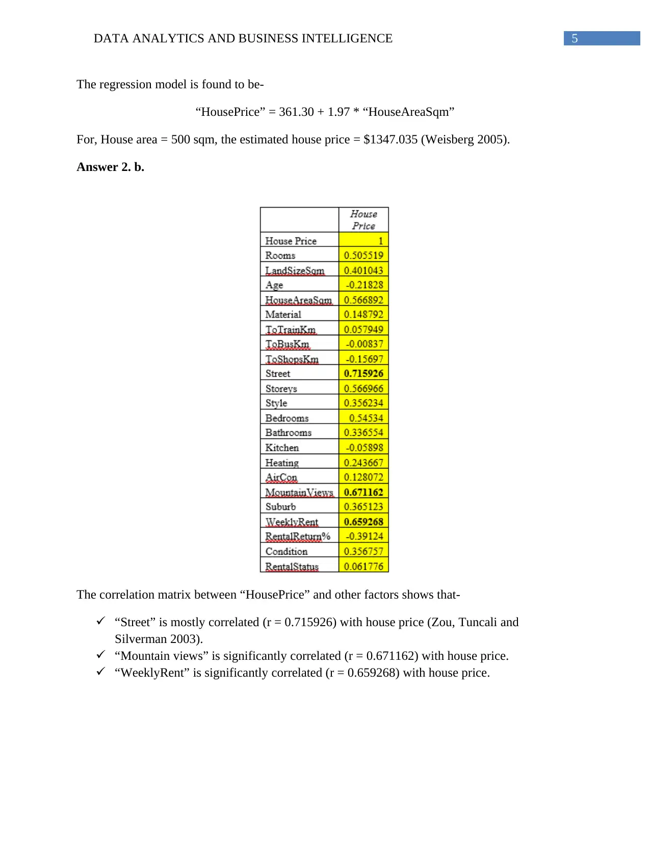
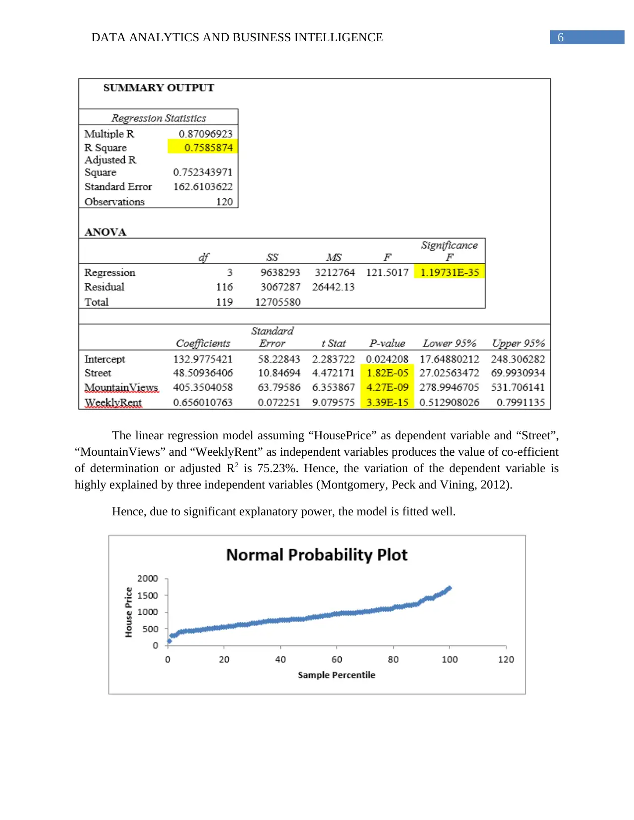
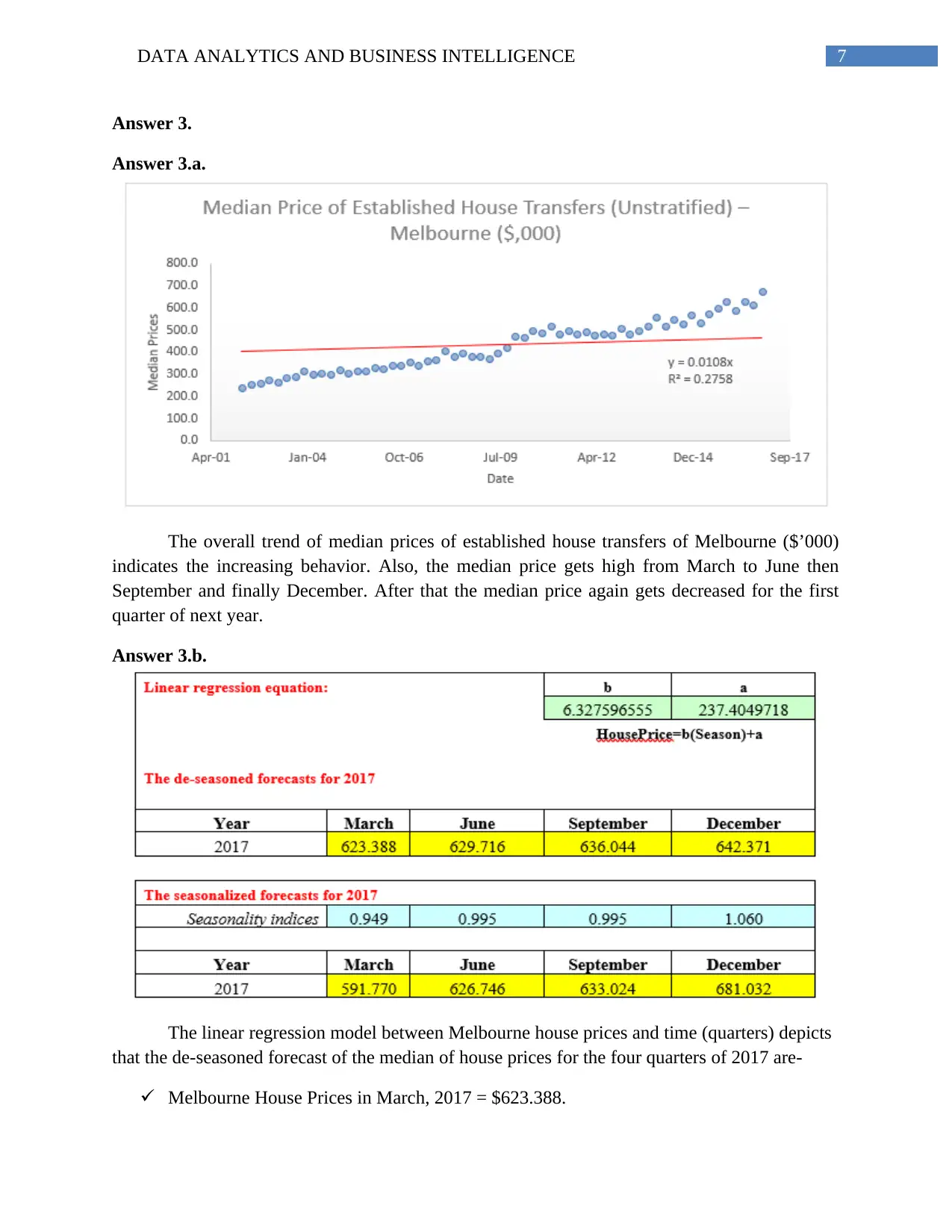
This document presents a detailed solution to a data analytics and business intelligence assignment. It begins with an analysis of house prices across different suburbs using cross-tabulation, followed by an examination of relationships between house prices and factors like land size, house area, and weekly rent through scatterplots and correlation analysis. The solution then employs linear regression models to estimate house prices based on house area and identifies the factors most correlated with house prices. Finally, the assignment addresses time series analysis, examining trends in Melbourne house prices and using linear regression to forecast future median prices for different quarters, both with and without seasonal adjustments. The solution includes relevant references to support the findings.

DATA ANALYTICS AND BUSINESS INTELLIGENCE
Data Analytics and Business Intelligence
Name of the student:
Name of the university:
Course ID:

1DATA ANALYTICS AND BUSINESS INTELLIGENCE
Table of Contents
Answer 1..........................................................................................................................................2
Answer 1. a..................................................................................................................................2
Answer 1. b..................................................................................................................................2
Answer 1.c...................................................................................................................................4
Answer 2..........................................................................................................................................4
Answer 2.a...................................................................................................................................4
Answer 2. b..................................................................................................................................5
Answer 3..........................................................................................................................................8
Answer 3.a...................................................................................................................................8
Answer 3.b...................................................................................................................................8
References:....................................................................................................................................10

2DATA ANALYTICS AND BUSINESS INTELLIGENCE
Answer 1.
Answer 1. a.
The cross-tabulation of house prices and suburb types indicates that total price of houses
is maximum for suburb 3 followed by suburb 1. The least total of houses is observed in case of
suburb 2. On an average, the price of houses is least in suburb 1 and highest in suburb 3.
Answer 1. b.
The scatterplot of size of land in square meters with respect to house price shows that-
 The linear relationship of these two factors is weak and positive (r2 = 18.43%).
 The non-linear relationship (polynomial pattern) between these two factors are weak and
insignificant (r2 = 3.1%).

3DATA ANALYTICS AND BUSINESS INTELLIGENCE
The scatterplot of size of house in square meters with respect to house price shows that-
 The linear relationship of these two factors is moderate and positive (r2 = 31.84%)
(Levine et al. 1999).
 The non-linear relationship (polynomial pattern) between these two factors are weak and
insignificant (r2 = 18.55%).
The scatterplot of size of weekly rent with respect to house price shows that-
 The linear relationship of these two factors is moderate and positive (r2 = 43.56%).
 The non-linear relationship (polynomial pattern) between these two factors are moderate
(r2 = 32.43%).

4DATA ANALYTICS AND BUSINESS INTELLIGENCE
Answer 1.c.
As per the values of coefficient of determinations (r2), the weekly rent has highest
association with house price. That is house price is mostly described by weekly rent rather than
land size (sqm) and house area (sqm).
Answer 2.
Answer 2.a.
The linear regression helps find out the estimated value of house prices with respect to
house area (sqm).

5DATA ANALYTICS AND BUSINESS INTELLIGENCE
The regression model is found to be-
“HousePrice” = 361.30 + 1.97 * “HouseAreaSqm”
For, House area = 500 sqm, the estimated house price = $1347.035 (Weisberg 2005).
Answer 2. b.
The correlation matrix between “HousePrice” and other factors shows that-
 “Street” is mostly correlated (r = 0.715926) with house price (Zou, Tuncali and
Silverman 2003).
 “Mountain views” is significantly correlated (r = 0.671162) with house price.
 “WeeklyRent” is significantly correlated (r = 0.659268) with house price.

6DATA ANALYTICS AND BUSINESS INTELLIGENCE
The linear regression model assuming “HousePrice” as dependent variable and “Street”,
“MountainViews” and “WeeklyRent” as independent variables produces the value of co-efficient
of determination or adjusted R2 is 75.23%. Hence, the variation of the dependent variable is
highly explained by three independent variables (Montgomery, Peck and Vining, 2012).
Hence, due to significant explanatory power, the model is fitted well.

7DATA ANALYTICS AND BUSINESS INTELLIGENCE
Answer 3.
Answer 3.a.
The overall trend of median prices of established house transfers of Melbourne ($’000)
indicates the increasing behavior. Also, the median price gets high from March to June then
September and finally December. After that the median price again gets decreased for the first
quarter of next year.
Answer 3.b.
The linear regression model between Melbourne house prices and time (quarters) depicts
that the de-seasoned forecast of the median of house prices for the four quarters of 2017 are-
 Melbourne House Prices in March, 2017 = $623.388.

8DATA ANALYTICS AND BUSINESS INTELLIGENCE
 Melbourne House Prices in June, 2017 = $629.716.
 Melbourne House Prices in September, 2017 = $636.044.
 Melbourne House Prices in December, 2017 = $642.371.
The seasonalized forecasts the median house prices for the four quarters of 2017-
 Melbourne House Prices in March, 2017 = $591.77.
 Melbourne House Prices in June, 2017 = $626.746.
 Melbourne House Prices in September, 2017 = $633.024.
 Melbourne House Prices in December, 2017 = $681.032.

9DATA ANALYTICS AND BUSINESS INTELLIGENCE
References:
Levine, D.M., Berenson, M.L., Stephan, D. and Lysell, D., 1999. Statistics for managers using
Microsoft Excel (Vol. 660). Upper Saddle River, NJ: Prentice Hall.
Montgomery, D.C., Peck, E.A. and Vining, G.G., 2012. Introduction to linear regression
analysis (Vol. 821). John Wiley & Sons.
Weisberg, S., 2005. Applied linear regression (Vol. 528). John Wiley & Sons.
Zou, K.H., Tuncali, K. and Silverman, S.G., 2003. Correlation and simple linear
regression. Radiology, 227(3), pp.617-628.