MGT723 Research Project: Data Analysis, Hypothesis Testing & Insights
VerifiedAdded on 2023/06/11
|15
|3138
|304
Report
AI Summary
This research project report presents a comprehensive analysis of data collected from 60 firms across various countries, focusing on carbon disclosure and stakeholder theory. The report details the data collection process, including the use of secondary data and random sampling. It includes descriptive statistics, chi-square tests, correlation analysis, and regression analysis to examine the relationships between variables. The findings discuss the impact of independent variables on disclosure scores, limitations of the study, and opportunities for future research. The assignment is available on Desklib, a platform offering a wide range of study tools and solved assignments for students.
Research Project
Contents
Data Collection............................................................................................................................................1
Data analysis................................................................................................................................................2
Descriptive statistics................................................................................................................................2
Inferential analysis...................................................................................................................................9
Hypothesis testing.....................................................................................................................................13
Discussion..................................................................................................................................................14
Limitation..................................................................................................................................................14
Future Research........................................................................................................................................14
References.................................................................................................................................................15
Data Collection
Data collection is one of the most important part of every research. There are broadly two types
of data which are used for the research. The first one is the primary data, which is also known as
the first hand data. The primary data are those data which are collected by the researcher as per
the requirement of the research. The major techniques used for data collection are the primary
survey (which is used to collect the quantitative data), personal interview (which is used to
collect the qualitative data). To collect the quantitative data the close end questionnaire is used
whereas for the qualitative data collection the open ended questionnaire is used.
The second type of the data which is used for the research is the secondary data. This type of
data is collected by someone else for different purpose. The major sources of the secondary data
includes the published journals, books, government data center, company reports etc. The
secondary data is cheap as compared to the primary data(Cierniak and Reimann, 2011; Mangal
and Mangal, 2013; Rajasekar, Philominathan and Chinnathambi, 2013).
For the current research the secondary data has been used. The data has been collected for 60
different firms situated in different countries around the world. The companies has been selected
from the master data set and the selection of the companies from the master data was random.
The random sampling has been used, so the results from the analysis can be generalized. Once
the sample was selected the data cleaning process has been conducted which included identifying
the missing values and the also the identification of the outliers. The missing values were
recoded so that the results are not affected. Once the data cleaning process was completed the
data was exported to SPSS and the further analysis was conducted(Armstrong, 2012; George,
Seals and Aban, 2014; Monem A Mohammed, 2014).
Paraphrase This Document
Need a fresh take? Get an instant paraphrase of this document with our AI Paraphraser
Data analysis
Data analysis has been conducted in two different ways. In the first section the results from the
descriptive analysis has been shown and in the next section the results from the inferential
analysis has been shown which includes the chi square test, correlation analysis and the
regression analysis.
Descriptive statistics
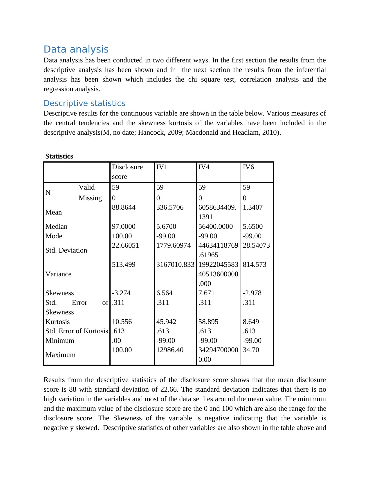
Descriptive results for the continuous variable are shown in the table below. Various measures of
the central tendencies and the skewness kurtosis of the variables have been included in the
descriptive analysis(M, no date; Hancock, 2009; Macdonald and Headlam, 2010).
Statistics
Disclosure
score
IV1 IV4 IV6
N Valid 59 59 59 59
Missing 0 0 0 0
Mean 88.8644 336.5706 6058634409.
1391
1.3407
Median 97.0000 5.6700 56400.0000 5.6500
Mode 100.00 -99.00 -99.00 -99.00
Std. Deviation 22.66051 1779.60974 44634118769
.61965
28.54073
Variance
513.499 3167010.833 19922045583
40513600000
.000
814.573
Skewness -3.274 6.564 7.671 -2.978
Std. Error of
Skewness
.311 .311 .311 .311
Kurtosis 10.556 45.942 58.895 8.649
Std. Error of Kurtosis .613 .613 .613 .613
Minimum .00 -99.00 -99.00 -99.00
Maximum 100.00 12986.40 34294700000
0.00
34.70
Results from the descriptive statistics of the disclosure score shows that the mean disclosure
score is 88 with standard deviation of 22.66. The standard deviation indicates that there is no
high variation in the variables and most of the data set lies around the mean value. The minimum
and the maximum value of the disclosure score are the 0 and 100 which are also the range for the
disclosure score. The Skewness of the variable is negative indicating that the variable is
negatively skewed. Descriptive statistics of other variables are also shown in the table above and
Data analysis has been conducted in two different ways. In the first section the results from the
descriptive analysis has been shown and in the next section the results from the inferential
analysis has been shown which includes the chi square test, correlation analysis and the
regression analysis.
Descriptive statistics
Descriptive results for the continuous variable are shown in the table below. Various measures of
the central tendencies and the skewness kurtosis of the variables have been included in the
descriptive analysis(M, no date; Hancock, 2009; Macdonald and Headlam, 2010).
Statistics
Disclosure
score
IV1 IV4 IV6
N Valid 59 59 59 59
Missing 0 0 0 0
Mean 88.8644 336.5706 6058634409.
1391
1.3407
Median 97.0000 5.6700 56400.0000 5.6500
Mode 100.00 -99.00 -99.00 -99.00
Std. Deviation 22.66051 1779.60974 44634118769
.61965
28.54073
Variance
513.499 3167010.833 19922045583
40513600000
.000
814.573
Skewness -3.274 6.564 7.671 -2.978
Std. Error of
Skewness
.311 .311 .311 .311
Kurtosis 10.556 45.942 58.895 8.649
Std. Error of Kurtosis .613 .613 .613 .613
Minimum .00 -99.00 -99.00 -99.00
Maximum 100.00 12986.40 34294700000
0.00
34.70
Results from the descriptive statistics of the disclosure score shows that the mean disclosure
score is 88 with standard deviation of 22.66. The standard deviation indicates that there is no
high variation in the variables and most of the data set lies around the mean value. The minimum
and the maximum value of the disclosure score are the 0 and 100 which are also the range for the
disclosure score. The Skewness of the variable is negative indicating that the variable is
negatively skewed. Descriptive statistics of other variables are also shown in the table above and
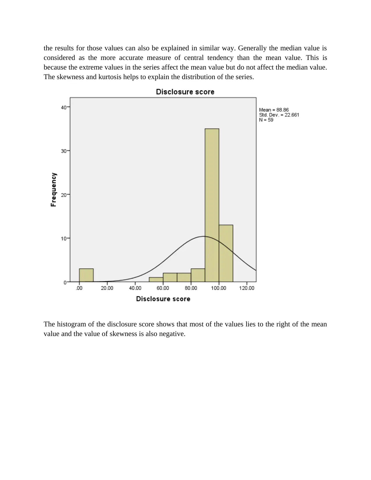
the results for those values can also be explained in similar way. Generally the median value is
considered as the more accurate measure of central tendency than the mean value. This is
because the extreme values in the series affect the mean value but do not affect the median value.
The skewness and kurtosis helps to explain the distribution of the series.
The histogram of the disclosure score shows that most of the values lies to the right of the mean
value and the value of skewness is also negative.
⊘ This is a preview!⊘
Do you want full access?
Subscribe today to unlock all pages.
Trusted by 1+ million students worldwide
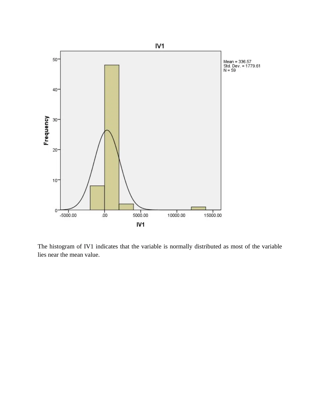
The histogram of IV1 indicates that the variable is normally distributed as most of the variable
lies near the mean value.
lies near the mean value.
Paraphrase This Document
Need a fresh take? Get an instant paraphrase of this document with our AI Paraphraser
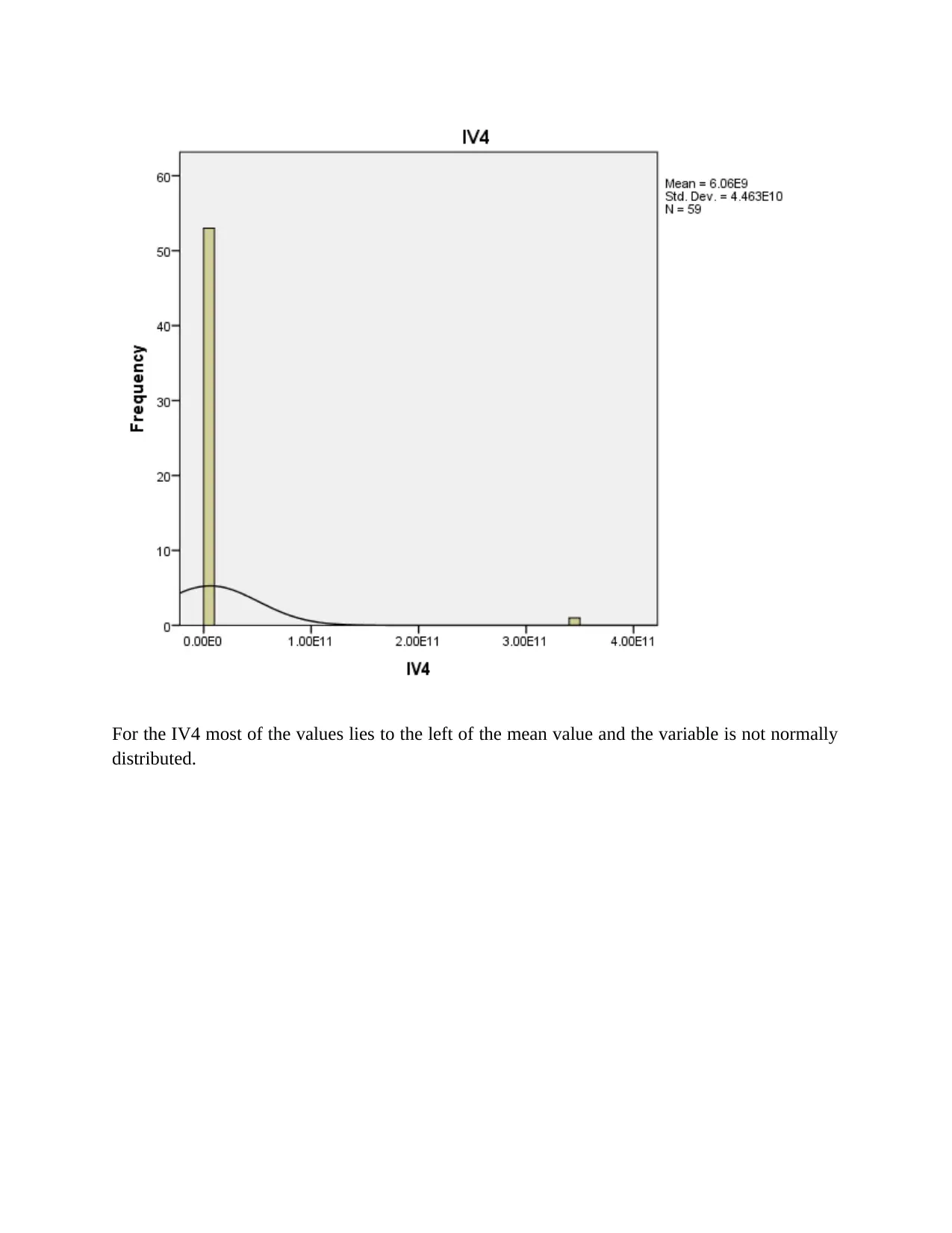
For the IV4 most of the values lies to the left of the mean value and the variable is not normally
distributed.
distributed.
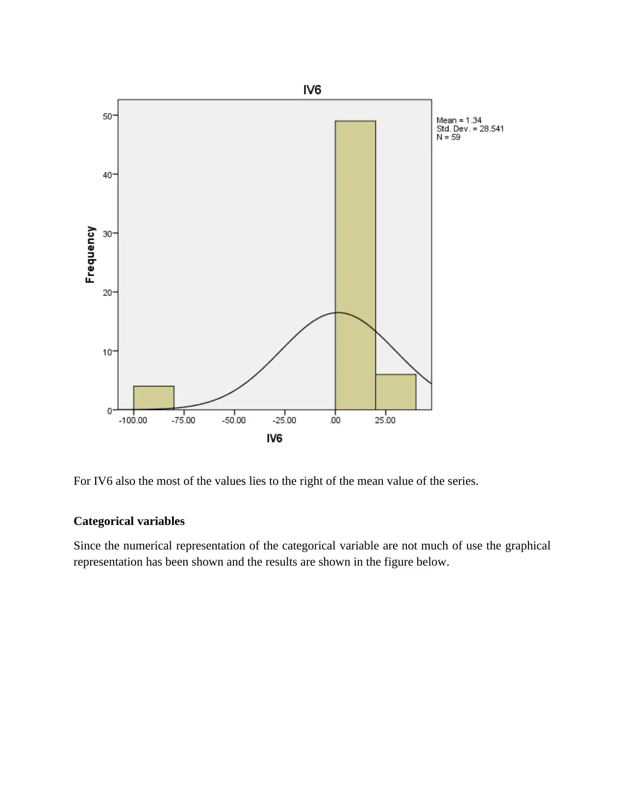
For IV6 also the most of the values lies to the right of the mean value of the series.
Categorical variables
Since the numerical representation of the categorical variable are not much of use the graphical
representation has been shown and the results are shown in the figure below.
Categorical variables
Since the numerical representation of the categorical variable are not much of use the graphical
representation has been shown and the results are shown in the figure below.
⊘ This is a preview!⊘
Do you want full access?
Subscribe today to unlock all pages.
Trusted by 1+ million students worldwide
12%
17%
22%14%
10%
10%
7% 8%
Industry
Financials
IT
industrials
Consumer Discretionary
materials
Consumer staples
Health care
others
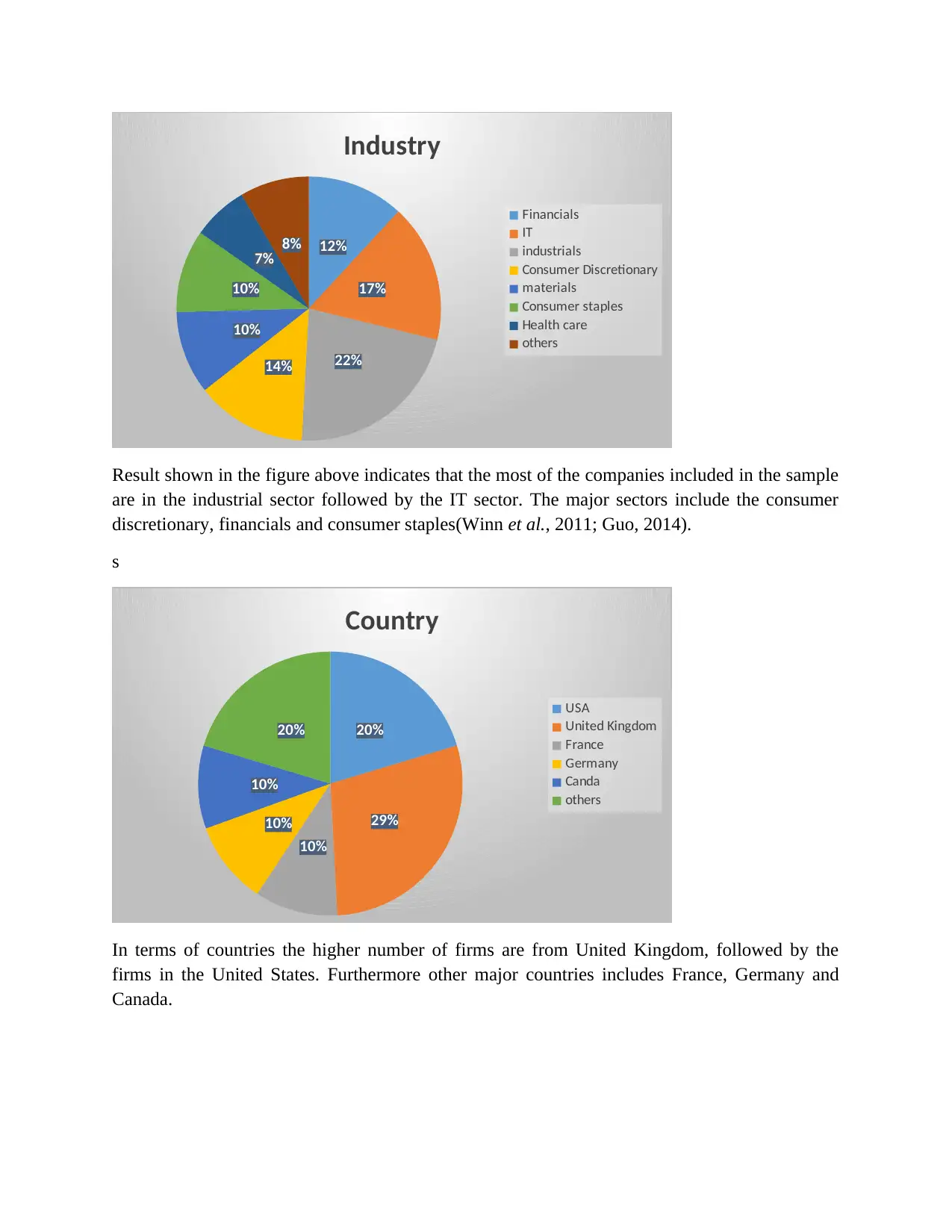
Result shown in the figure above indicates that the most of the companies included in the sample
are in the industrial sector followed by the IT sector. The major sectors include the consumer
discretionary, financials and consumer staples(Winn et al., 2011; Guo, 2014).
s
20%
29%
10%
10%
10%
20%
Country
USA
United Kingdom
France
Germany
Canda
others
In terms of countries the higher number of firms are from United Kingdom, followed by the
firms in the United States. Furthermore other major countries includes France, Germany and
Canada.
17%
22%14%
10%
10%
7% 8%
Industry
Financials
IT
industrials
Consumer Discretionary
materials
Consumer staples
Health care
others
Result shown in the figure above indicates that the most of the companies included in the sample
are in the industrial sector followed by the IT sector. The major sectors include the consumer
discretionary, financials and consumer staples(Winn et al., 2011; Guo, 2014).
s
20%
29%
10%
10%
10%
20%
Country
USA
United Kingdom
France
Germany
Canda
others
In terms of countries the higher number of firms are from United Kingdom, followed by the
firms in the United States. Furthermore other major countries includes France, Germany and
Canada.
Paraphrase This Document
Need a fresh take? Get an instant paraphrase of this document with our AI Paraphraser
49%51%
IV3
other
full time
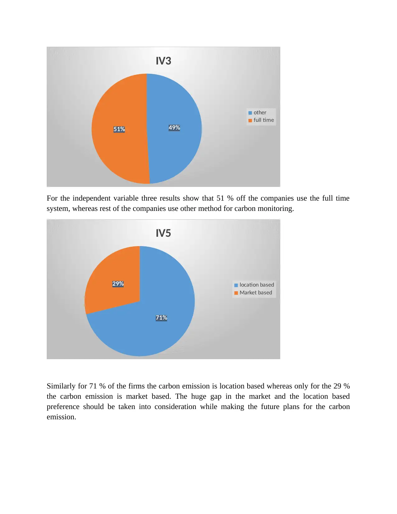
For the independent variable three results show that 51 % off the companies use the full time
system, whereas rest of the companies use other method for carbon monitoring.
71%
29%
IV5
location based
Market based
Similarly for 71 % of the firms the carbon emission is location based whereas only for the 29 %
the carbon emission is market based. The huge gap in the market and the location based
preference should be taken into consideration while making the future plans for the carbon
emission.
IV3
other
full time
For the independent variable three results show that 51 % off the companies use the full time
system, whereas rest of the companies use other method for carbon monitoring.
71%
29%
IV5
location based
Market based
Similarly for 71 % of the firms the carbon emission is location based whereas only for the 29 %
the carbon emission is market based. The huge gap in the market and the location based
preference should be taken into consideration while making the future plans for the carbon
emission.
71%
29%
IV7
decrease
Increase
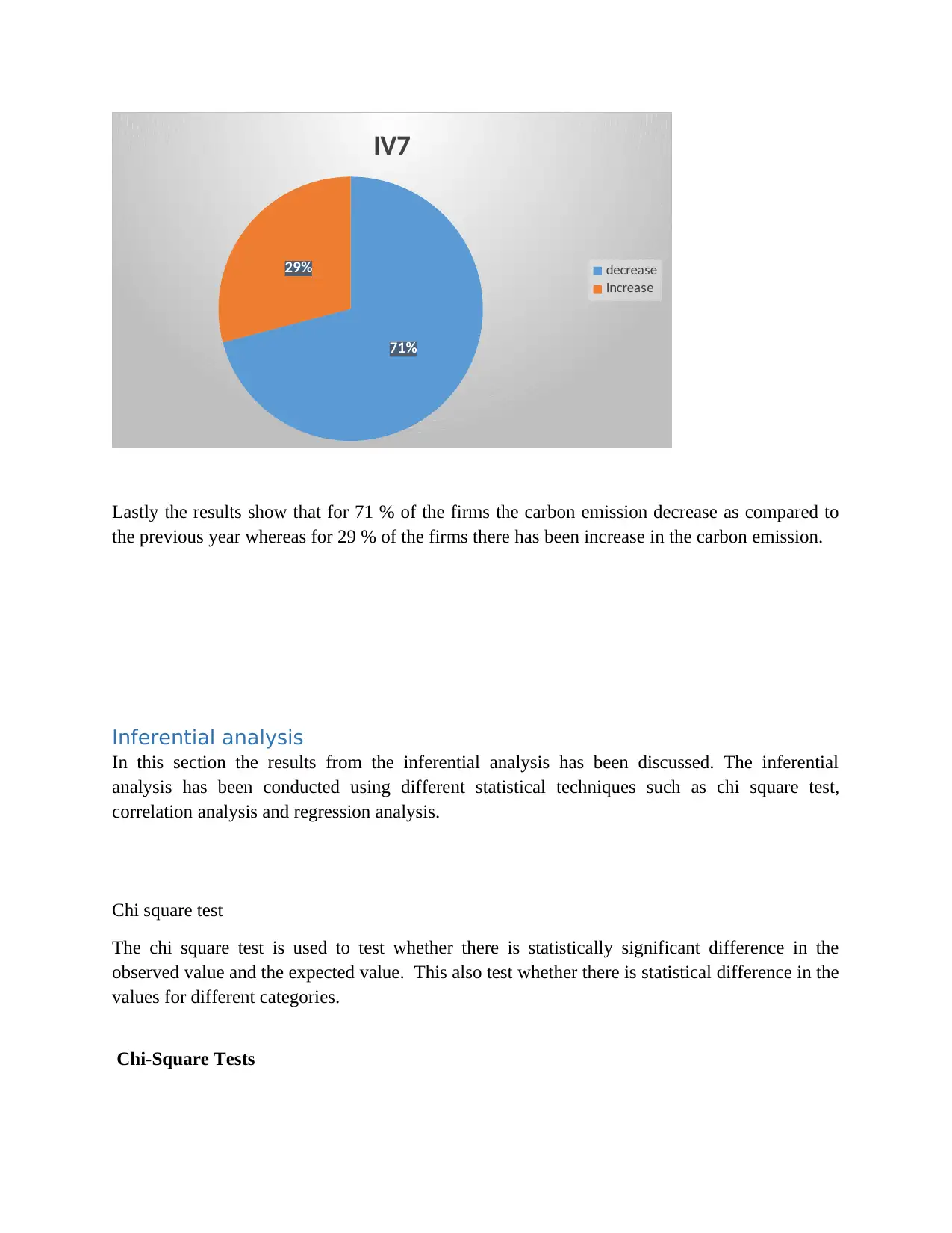
Lastly the results show that for 71 % of the firms the carbon emission decrease as compared to
the previous year whereas for 29 % of the firms there has been increase in the carbon emission.
Inferential analysis
In this section the results from the inferential analysis has been discussed. The inferential
analysis has been conducted using different statistical techniques such as chi square test,
correlation analysis and regression analysis.
Chi square test
The chi square test is used to test whether there is statistically significant difference in the
observed value and the expected value. This also test whether there is statistical difference in the
values for different categories.
Chi-Square Tests
29%
IV7
decrease
Increase
Lastly the results show that for 71 % of the firms the carbon emission decrease as compared to
the previous year whereas for 29 % of the firms there has been increase in the carbon emission.
Inferential analysis
In this section the results from the inferential analysis has been discussed. The inferential
analysis has been conducted using different statistical techniques such as chi square test,
correlation analysis and regression analysis.
Chi square test
The chi square test is used to test whether there is statistically significant difference in the
observed value and the expected value. This also test whether there is statistical difference in the
values for different categories.
Chi-Square Tests
⊘ This is a preview!⊘
Do you want full access?
Subscribe today to unlock all pages.
Trusted by 1+ million students worldwide
Value df Asymp. Sig.
(2-sided)
Pearson Chi-Square 100.296a 90 .215
Likelihood Ratio 85.454 90 .616
Linear-by-Linear
Association
1.618 1 .203
N of Valid Cases 59
a. 114 cells (100.0%) have expected count less than 5. The
minimum expected count is .10.
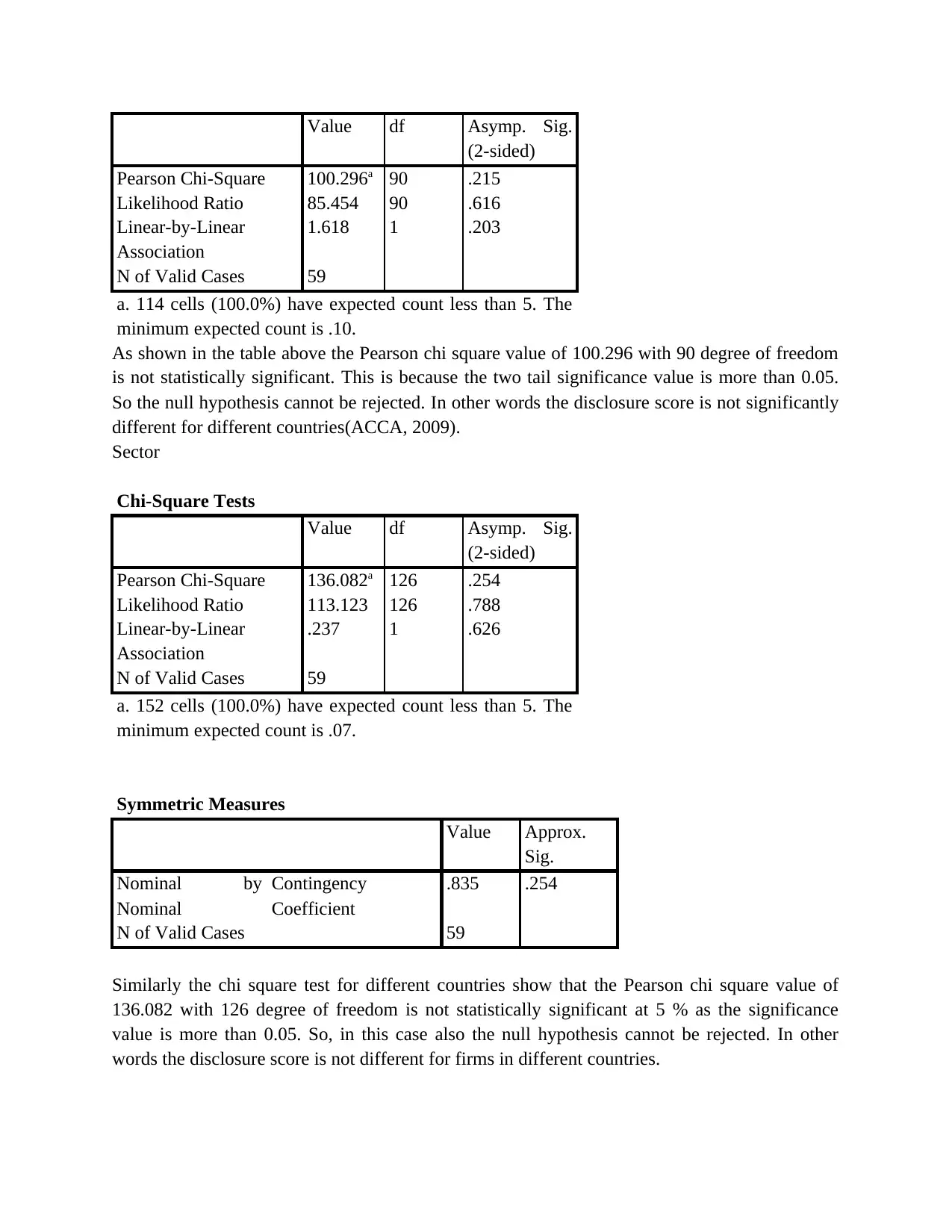
As shown in the table above the Pearson chi square value of 100.296 with 90 degree of freedom
is not statistically significant. This is because the two tail significance value is more than 0.05.
So the null hypothesis cannot be rejected. In other words the disclosure score is not significantly
different for different countries(ACCA, 2009).
Sector
Chi-Square Tests
Value df Asymp. Sig.
(2-sided)
Pearson Chi-Square 136.082a 126 .254
Likelihood Ratio 113.123 126 .788
Linear-by-Linear
Association
.237 1 .626
N of Valid Cases 59
a. 152 cells (100.0%) have expected count less than 5. The
minimum expected count is .07.
Symmetric Measures
Value Approx.
Sig.
Nominal by
Nominal
Contingency
Coefficient
.835 .254
N of Valid Cases 59
Similarly the chi square test for different countries show that the Pearson chi square value of
136.082 with 126 degree of freedom is not statistically significant at 5 % as the significance
value is more than 0.05. So, in this case also the null hypothesis cannot be rejected. In other
words the disclosure score is not different for firms in different countries.
(2-sided)
Pearson Chi-Square 100.296a 90 .215
Likelihood Ratio 85.454 90 .616
Linear-by-Linear
Association
1.618 1 .203
N of Valid Cases 59
a. 114 cells (100.0%) have expected count less than 5. The
minimum expected count is .10.
As shown in the table above the Pearson chi square value of 100.296 with 90 degree of freedom
is not statistically significant. This is because the two tail significance value is more than 0.05.
So the null hypothesis cannot be rejected. In other words the disclosure score is not significantly
different for different countries(ACCA, 2009).
Sector
Chi-Square Tests
Value df Asymp. Sig.
(2-sided)
Pearson Chi-Square 136.082a 126 .254
Likelihood Ratio 113.123 126 .788
Linear-by-Linear
Association
.237 1 .626
N of Valid Cases 59
a. 152 cells (100.0%) have expected count less than 5. The
minimum expected count is .07.
Symmetric Measures
Value Approx.
Sig.
Nominal by
Nominal
Contingency
Coefficient
.835 .254
N of Valid Cases 59
Similarly the chi square test for different countries show that the Pearson chi square value of
136.082 with 126 degree of freedom is not statistically significant at 5 % as the significance
value is more than 0.05. So, in this case also the null hypothesis cannot be rejected. In other
words the disclosure score is not different for firms in different countries.
Paraphrase This Document
Need a fresh take? Get an instant paraphrase of this document with our AI Paraphraser
Correlation analysis
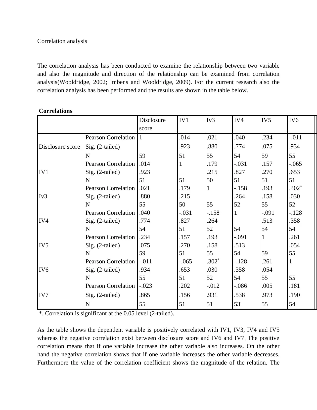
The correlation analysis has been conducted to examine the relationship between two variable
and also the magnitude and direction of the relationship can be examined from correlation
analysis(Wooldridge, 2002; Imbens and Wooldridge, 2009). For the current research also the
correlation analysis has been performed and the results are shown in the table below.
Correlations
Disclosure
score
IV1 Iv3 IV4 IV5 IV6 I
Disclosure score
Pearson Correlation 1 .014 .021 .040 .234 -.011 -
Sig. (2-tailed) .923 .880 .774 .075 .934 .
N 59 51 55 54 59 55 5
IV1
Pearson Correlation .014 1 .179 -.031 .157 -.065 .
Sig. (2-tailed) .923 .215 .827 .270 .653 .
N 51 51 50 51 51 51 5
Iv3
Pearson Correlation .021 .179 1 -.158 .193 .302* -
Sig. (2-tailed) .880 .215 .264 .158 .030 .
N 55 50 55 52 55 52 5
IV4
Pearson Correlation .040 -.031 -.158 1 -.091 -.128 -
Sig. (2-tailed) .774 .827 .264 .513 .358 .
N 54 51 52 54 54 54 5
IV5
Pearson Correlation .234 .157 .193 -.091 1 .261 .
Sig. (2-tailed) .075 .270 .158 .513 .054 .
N 59 51 55 54 59 55 5
IV6
Pearson Correlation -.011 -.065 .302* -.128 .261 1 .
Sig. (2-tailed) .934 .653 .030 .358 .054 .
N 55 51 52 54 55 55 5
IV7
Pearson Correlation -.023 .202 -.012 -.086 .005 .181 1
Sig. (2-tailed) .865 .156 .931 .538 .973 .190
N 55 51 51 53 55 54 5
*. Correlation is significant at the 0.05 level (2-tailed).
As the table shows the dependent variable is positively correlated with IV1, IV3, IV4 and IV5
whereas the negative correlation exist between disclosure score and IV6 and IV7. The positive
correlation means that if one variable increase the other variable also increases. On the other
hand the negative correlation shows that if one variable increases the other variable decreases.
Furthermore the value of the correlation coefficient shows the magnitude of the relation. The
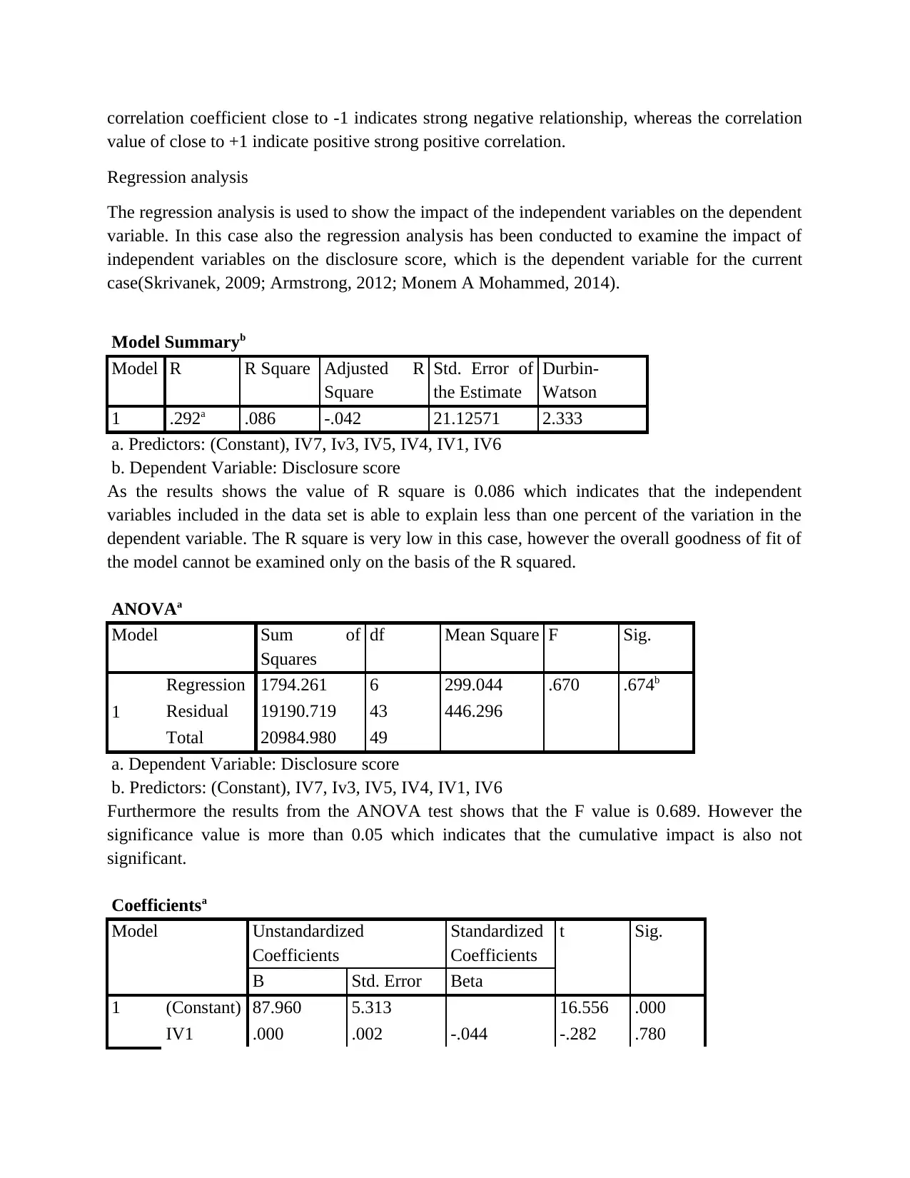
correlation coefficient close to -1 indicates strong negative relationship, whereas the correlation
value of close to +1 indicate positive strong positive correlation.
Regression analysis
The regression analysis is used to show the impact of the independent variables on the dependent
variable. In this case also the regression analysis has been conducted to examine the impact of
independent variables on the disclosure score, which is the dependent variable for the current
case(Skrivanek, 2009; Armstrong, 2012; Monem A Mohammed, 2014).
Model Summaryb
Model R R Square Adjusted R
Square
Std. Error of
the Estimate
Durbin-
Watson
1 .292a .086 -.042 21.12571 2.333
a. Predictors: (Constant), IV7, Iv3, IV5, IV4, IV1, IV6
b. Dependent Variable: Disclosure score
As the results shows the value of R square is 0.086 which indicates that the independent
variables included in the data set is able to explain less than one percent of the variation in the
dependent variable. The R square is very low in this case, however the overall goodness of fit of
the model cannot be examined only on the basis of the R squared.
ANOVAa
Model Sum of
Squares
df Mean Square F Sig.
1
Regression 1794.261 6 299.044 .670 .674b
Residual 19190.719 43 446.296
Total 20984.980 49
a. Dependent Variable: Disclosure score
b. Predictors: (Constant), IV7, Iv3, IV5, IV4, IV1, IV6
Furthermore the results from the ANOVA test shows that the F value is 0.689. However the
significance value is more than 0.05 which indicates that the cumulative impact is also not
significant.
Coefficientsa
Model Unstandardized
Coefficients
Standardized
Coefficients
t Sig.
B Std. Error Beta
1 (Constant) 87.960 5.313 16.556 .000
IV1 .000 .002 -.044 -.282 .780
⊘ This is a preview!⊘
Do you want full access?
Subscribe today to unlock all pages.
Trusted by 1+ million students worldwide
1 out of 15
Related Documents


Your All-in-One AI-Powered Toolkit for Academic Success.
+13062052269
info@desklib.com
Available 24*7 on WhatsApp / Email
![[object Object]](/_next/static/media/star-bottom.7253800d.svg)
Unlock your academic potential
Copyright © 2020–2026 A2Z Services. All Rights Reserved. Developed and managed by ZUCOL.