University Data Science: Assessment 4 - Data Analysis Report

This report presents a data analysis project utilizing South Australian household data from 2018, focusing on predicting household tenure types. The project employs two primary data analysis techniques: multivariate linear regression and k-means clustering. The dataset includes variables such as LGA name, tenure type, and various income brackets. The report details the application of both techniques using SPSS, including data preparation, descriptive statistics, hypothesis formulation, and model building. The linear regression analysis reveals a weak relationship between tenure type and the predictors, while the k-means clustering algorithm, optimized with k=3 clusters, provides better insights by grouping tenure types based on LDA names and total households. The report includes detailed results, ANOVA tables, and post-hoc analysis to validate the findings and compare the effectiveness of the two methods. The analysis concludes with recommendations based on the comparative performance of the techniques.

Running head: ASSESSMENT 4
ASSESSMENT 4
Name of the Student
Name of the University
Author Note

1ASSESSMENT 4
Executive summary:
Data analysis is a very useful technique to extract key insights from a raw data and to make
predictions or classifications based on the data. There are various data analysis techniques
that are used in various industries for solving business problems, decision making and
producing hidden insights from data and by using modern computing techniques the spread
and effectiveness of data analysis is expanding to approach more complicated problems year
after years. The two techniques of data analysis namely the multivariate linear regression and
clustering are applied on the south Australian household data of 2018 collected from the
corresponding website for predicting the tenure type of households and necessary
significance and validation of the predictions are made.

2ASSESSMENT 4
Table of Contents
Introduction:...............................................................................................................................3
Data analysis:.............................................................................................................................4
Conclusions and recommendations:.........................................................................................15
References:...............................................................................................................................16

3ASSESSMENT 4
Introduction:
In this particular project a suitable data is collected from the Australian government data
official website and two analysis techniques are applied on the data and results are compared.
In the dataset there are a total of six variables namely LGA Name, Tenure type, very low
income houses, low income houses and moderate income houses and Total houses. The total
number of South Australian households who are paying more than 30% of the total household
earnings are segregated in three income brackets which are very low (for less than $603 per
week), low income (for income between $603 to $964 per week) and moderate income (for
income between $965 to $1446 per week). There is also one Total variable that includes the
income groups as well as the people who do not fall under the groups but pays more than
30% of their income to households (Data.sa.gov.au 2020). The LGA name are the area name
of the corresponding households as defined by each state and Territory local government
department in 2016. The boundaries of LDA areas are constructed based on the allocations of
the mesh blocks and reviewed on annual basis. The variable tenure type is the type of those
particular households which includes following types.
1) Rented: Private and not stated
2) Rented: Other landlord
3) Rented: TOTAL
4) Other tenure types
5) Rented: Total
6) Total households
7) Being purchased (incl rent/buy)

4ASSESSMENT 4
The definitions of the tenure types in details can be found on the Australian government
website link as specified in the references sections.
Now, by data analysis with SPSS the objective is to find any relationship between the
variables Total households, their respective LDA names and corresponding tenure types. In
particular the tenure types are being predicted in terms of LDA names and Total households.
Hence, the interested variables for analysis are three with the number of instances or sample
size equal to 497. Now, as LDA names and tenure type are categorical variables, hence they
are first converted into numerical variable for analysis using SPSS automatic recoding
scheme. By the scheme tenure type is recoded from lowest value in alphabetical manner and
thus 7 tenures from ‘being purchased (incl rent/buy)’ to ‘Total households’ are recoded from
1 to 7. Also, the same scheme is applied for LDA names where areas ‘Adelaide (C)’ to
‘Yorke Peninsula (DC)’ are recoded from 1 to 71.
Data analysis:
Now, the collected data of 497 sample size has no missing values and thus no filtering of the
data is required before analysis. Two methods of prediction analysis is performed with the
data which are linear regression analysis as a simplistic prediction technique and the
clustering analysis with k-means algorithm (Ho 2017). In both cases the tenure type is
considered as the dependent variable which is predicted in terms of predictors LDA name and
Total (the total number of households paying over 30% of earnings). Now, before performing
the two prediction methods the descriptive statistics of the variables are calculated in SPSS.
Descriptive statistics of variables:
Descriptive Statistics
N Minimum Maximum Mean Std. Deviation

5ASSESSMENT 4
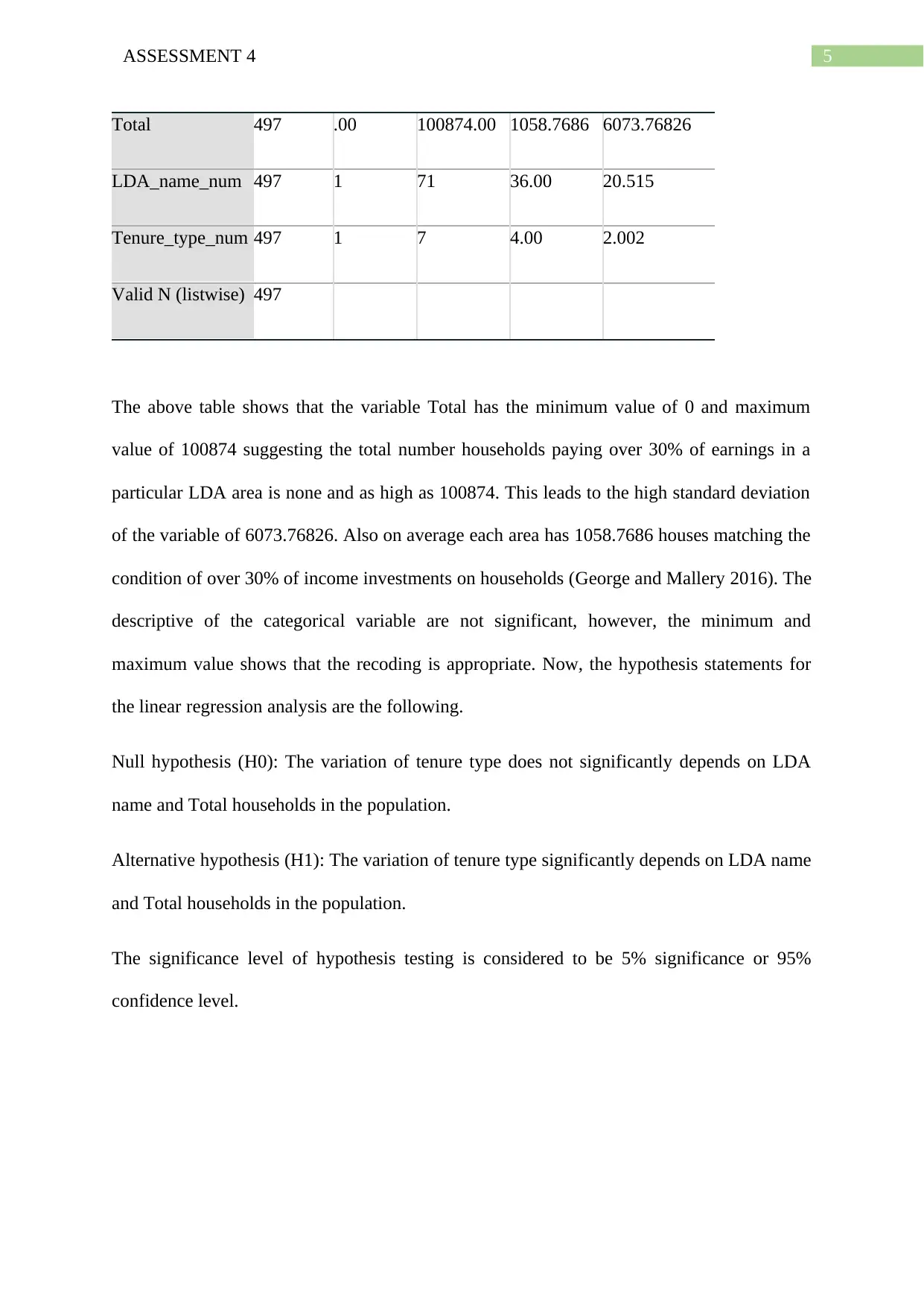
Total 497 .00 100874.00 1058.7686 6073.76826
LDA_name_num 497 1 71 36.00 20.515
Tenure_type_num 497 1 7 4.00 2.002
Valid N (listwise) 497
The above table shows that the variable Total has the minimum value of 0 and maximum
value of 100874 suggesting the total number households paying over 30% of earnings in a
particular LDA area is none and as high as 100874. This leads to the high standard deviation
of the variable of 6073.76826. Also on average each area has 1058.7686 houses matching the
condition of over 30% of income investments on households (George and Mallery 2016). The
descriptive of the categorical variable are not significant, however, the minimum and
maximum value shows that the recoding is appropriate. Now, the hypothesis statements for
the linear regression analysis are the following.
Null hypothesis (H0): The variation of tenure type does not significantly depends on LDA
name and Total households in the population.
Alternative hypothesis (H1): The variation of tenure type significantly depends on LDA name
and Total households in the population.
The significance level of hypothesis testing is considered to be 5% significance or 95%
confidence level.

6ASSESSMENT 4
Prediction by linear regression:
In linear regression a linear trend line is fitted to the data which minimizes the sum of square
error between the given data points and the line. The general equation of the multivariate
regression is given by,
Y = a + b1*X1 + b2*X2 +…+ bk*Xk + e
Here, X1,X2,…,Xk are the independent variables, Y is dependent variable and e is the error
term in prediction which is also referred as residual. Now, in this case the number of
predictors is two and hence the formula reduces to
y = a + b1*X1 + b2*X2
For a single predictor variable case the slope coefficients are given by,
b = ∑ xy
∑ x2
a = mean(y) – b*mean(x)
Now, for the two variable case the slope coefficients will be,
b1 = ¿
b2 = ¿
a = mean(y) – b1*mean(x1) – b2*mean(x2)
Now, in SPSS the two variable linear regression model is built as given below.
Variables Entered/Removeda
Model
Variables
Entered
Variables
Removed Method

7ASSESSMENT 4
1 LDA_name_n
um, Totalb
. Enter
a. Dependent Variable: Tenure_type_num
b. All requested variables entered.
Model Summaryb
Model R R Square
Adjusted R
Square
Std. Error of
the Estimate
Durbin-
Watson
1 .104a .011 .007 1.995 3.690
a. Predictors: (Constant), LDA_name_num, Total
b. Dependent Variable: Tenure_type_num
Coefficientsa
Model
Unstandardized
Coefficients
Standardized
Coefficients
t Sig.B Std. Error Beta
1 (Constant) 3.996 .181 22.087 .000
Total 3.427E-5 .000 .104 2.314 .021
LDA_name_num -.001 .004 -.009 -.204 .838
a. Dependent Variable: Tenure_type_num

8ASSESSMENT 4
Residuals Statisticsa
Minimum Maximum Mean Std. Deviation N
Predicted Value 3.93 7.40 4.00 .207 497
Residual -4.298 3.065 .000 1.991 497
Std. Predicted Value-.326 16.416 .000 1.000 497
Std. Residual -2.154 1.536 .000 .998 497
a. Dependent Variable: Tenure_type_num
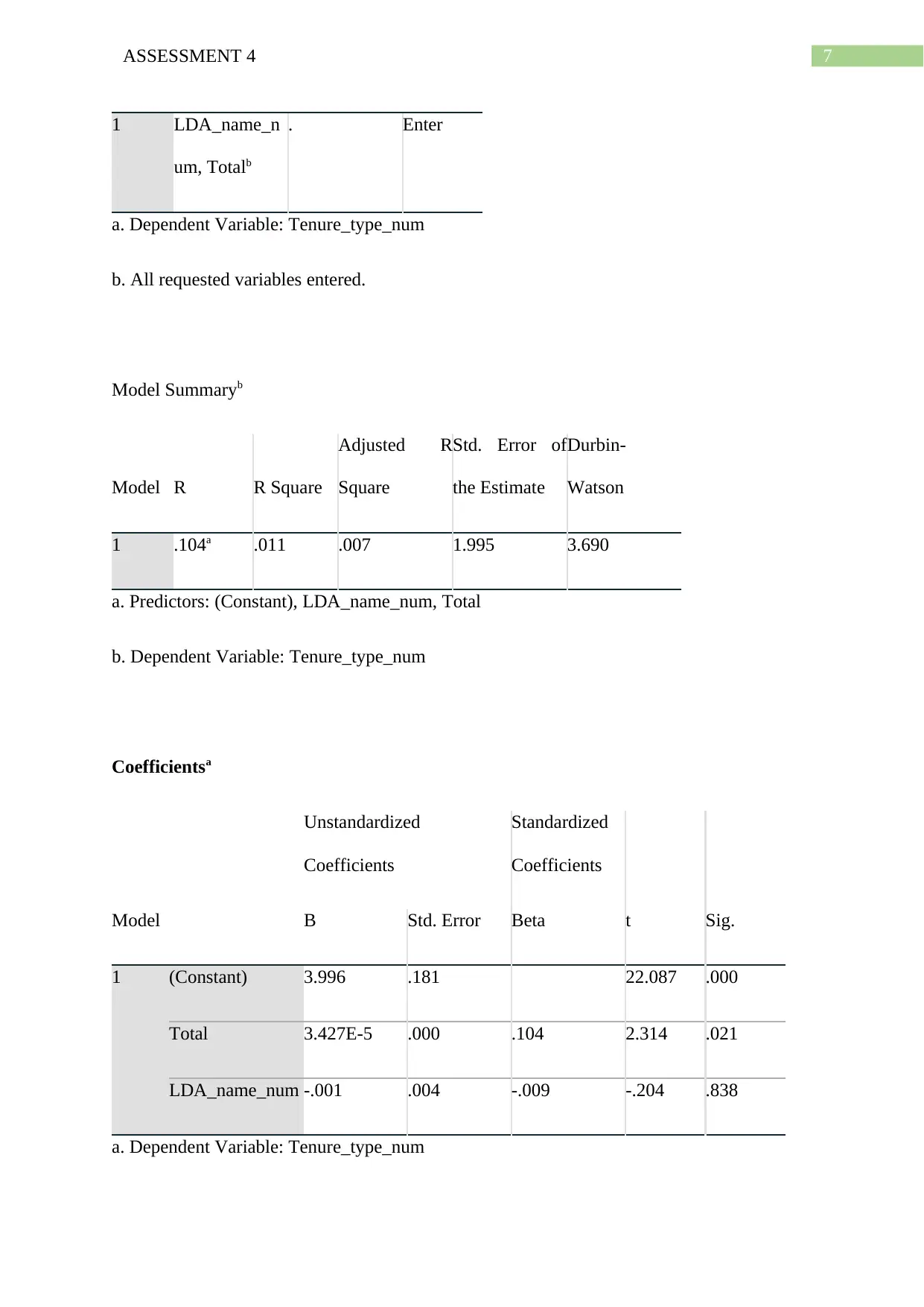
Now, by the method of linear regression analysis it is evident that the relationship between
the dependent and its predictors are not strong as the adjusted R2 or coefficient of
determination value is very low (0.01) and so as the correlation coefficient. The prediction
model is given by the following equation.
Tenure_type_num = 3.996 + 3.427∗10−5 – 0.001* LDA_name_num
The p value of the predictor Total is significant as the value is under 0.05, however the
predictor LDA_name_num is not significant. The overall model is not significant as indicated
the by the high durbin-watson value as well as the R2 which shows very less percentage of
variation in tenure type is explained by variation of LDA name and Total number of
household satisfying condition (Wathan et al. 2019). Hence, there is not enough evidence to
reject the null hypothesis and thus it can be concluded by the linear regression is that the
variation of tenure type does not significantly depends on LDA name and Total households in
the population.

9ASSESSMENT 4
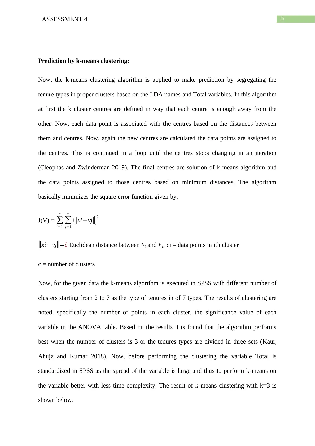
Prediction by k-means clustering:
Now, the k-means clustering algorithm is applied to make prediction by segregating the
tenure types in proper clusters based on the LDA names and Total variables. In this algorithm
at first the k cluster centres are defined in way that each centre is enough away from the
other. Now, each data point is associated with the centres based on the distances between
them and centres. Now, again the new centres are calculated the data points are assigned to
the centres. This is continued in a loop until the centres stops changing in an iteration
(Cleophas and Zwinderman 2019). The final centres are solution of k-means algorithm and
the data points assigned to those centres based on minimum distances. The algorithm
basically minimizes the square error function given by,
J(V) = ∑
i=1
c
∑
j=1
ci
(||xi−vj||)2
||xi−vj||=¿ Euclidean distance between xi and v j, ci = data points in ith cluster
c = number of clusters
Now, for the given data the k-means algorithm is executed in SPSS with different number of
clusters starting from 2 to 7 as the type of tenures in of 7 types. The results of clustering are
noted, specifically the number of points in each cluster, the significance value of each
variable in the ANOVA table. Based on the results it is found that the algorithm performs
best when the number of clusters is 3 or the tenures types are divided in three sets (Kaur,
Ahuja and Kumar 2018). Now, before performing the clustering the variable Total is
standardized in SPSS as the spread of the variable is large and thus to perform k-means on
the variable better with less time complexity. The result of k-means clustering with k=3 is
shown below.

10ASSESSMENT 4
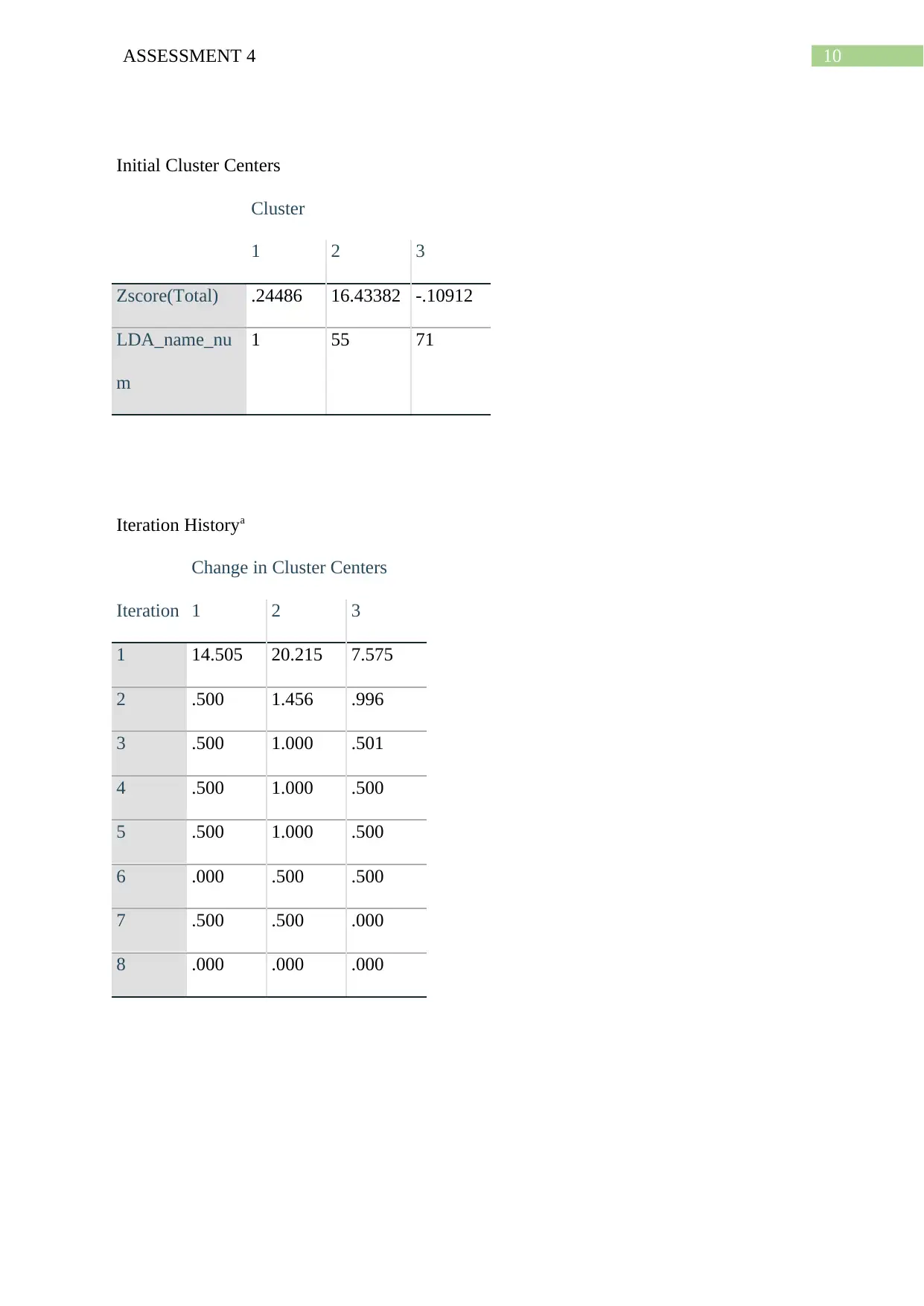
Initial Cluster Centers
Cluster
1 2 3
Zscore(Total) .24486 16.43382 -.10912
LDA_name_nu
m
1 55 71
Iteration Historya
Iteration
Change in Cluster Centers
1 2 3
1 14.505 20.215 7.575
2 .500 1.456 .996
3 .500 1.000 .501
4 .500 1.000 .500
5 .500 1.000 .500
6 .000 .500 .500
7 .500 .500 .000
8 .000 .000 .000

11ASSESSMENT 4
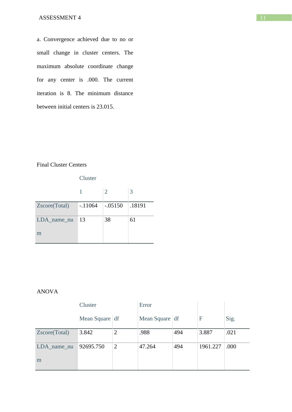
a. Convergence achieved due to no or
small change in cluster centers. The
maximum absolute coordinate change
for any center is .000. The current
iteration is 8. The minimum distance
between initial centers is 23.015.
Final Cluster Centers
Cluster
1 2 3
Zscore(Total) -.11064 -.05150 .18191
LDA_name_nu
m
13 38 61
ANOVA
Cluster Error
F Sig.Mean Square df Mean Square df
Zscore(Total) 3.842 2 .988 494 3.887 .021
LDA_name_nu
m
92695.750 2 47.264 494 1961.227 .000