Statistical Data Analysis: Hypothesis Testing and Regression Analysis

This assignment delves into various statistical techniques, including hypothesis testing, ANOVA, t-tests, and regression analysis, to analyze different datasets. It begins with an ANOVA test to compare the average TMA scores across three courses at SUSS, concluding no significant difference. The assignment then explores a one-tailed t-test to determine if a new swimming method improves timing, finding no significant improvement. It further elucidates the differences between sampling error and standard error, as well as interval and ratio scales, and statistics and parameters. The assignment also examines the correlation between academic performance and family closeness, finding a positive correlation. Finally, it uses simple linear regression to estimate grade point average based on time spent with family and conducts an independent samples t-test to compare anger propensity scores between males and females, revealing significant differences.

Data Analysis
1

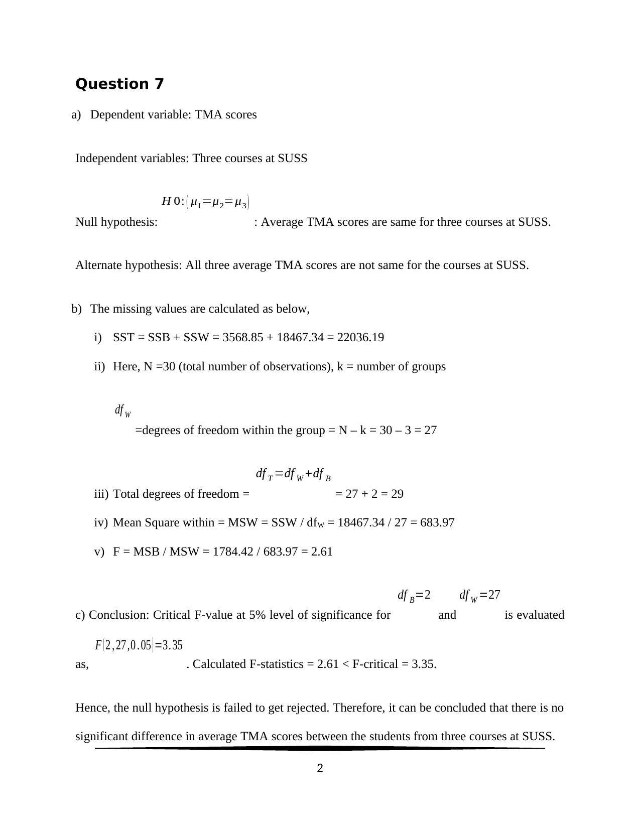
Question 7
a) Dependent variable: TMA scores
Independent variables: Three courses at SUSS
Null hypothesis:
H 0: ( μ1=μ2=μ3 )
: Average TMA scores are same for three courses at SUSS.
Alternate hypothesis: All three average TMA scores are not same for the courses at SUSS.
b) The missing values are calculated as below,
i) SST = SSB + SSW = 3568.85 + 18467.34 = 22036.19
ii) Here, N =30 (total number of observations), k = number of groups
df W
=degrees of freedom within the group = N – k = 30 – 3 = 27
iii) Total degrees of freedom =
df T =df W +df B
= 27 + 2 = 29
iv) Mean Square within = MSW = SSW / dfW = 18467.34 / 27 = 683.97
v) F = MSB / MSW = 1784.42 / 683.97 = 2.61
c) Conclusion: Critical F-value at 5% level of significance for
df B=2
and
df W =27
is evaluated
as,
F ( 2 , 27 ,0 . 05 ) =3. 35
. Calculated F-statistics = 2.61 < F-critical = 3.35.
Hence, the null hypothesis is failed to get rejected. Therefore, it can be concluded that there is no
significant difference in average TMA scores between the students from three courses at SUSS.
2

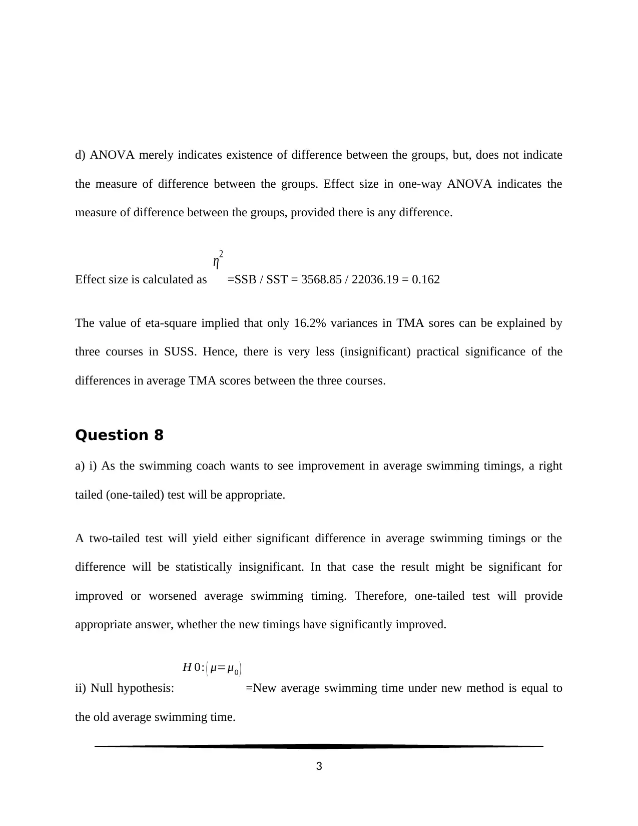
d) ANOVA merely indicates existence of difference between the groups, but, does not indicate
the measure of difference between the groups. Effect size in one-way ANOVA indicates the
measure of difference between the groups, provided there is any difference.
Effect size is calculated as
η2
=SSB / SST = 3568.85 / 22036.19 = 0.162
The value of eta-square implied that only 16.2% variances in TMA sores can be explained by
three courses in SUSS. Hence, there is very less (insignificant) practical significance of the
differences in average TMA scores between the three courses.
Question 8
a) i) As the swimming coach wants to see improvement in average swimming timings, a right
tailed (one-tailed) test will be appropriate.
A two-tailed test will yield either significant difference in average swimming timings or the
difference will be statistically insignificant. In that case the result might be significant for
improved or worsened average swimming timing. Therefore, one-tailed test will provide
appropriate answer, whether the new timings have significantly improved.
ii) Null hypothesis:
H 0: ( μ=μ0 )
=New average swimming time under new method is equal to
the old average swimming time.
3

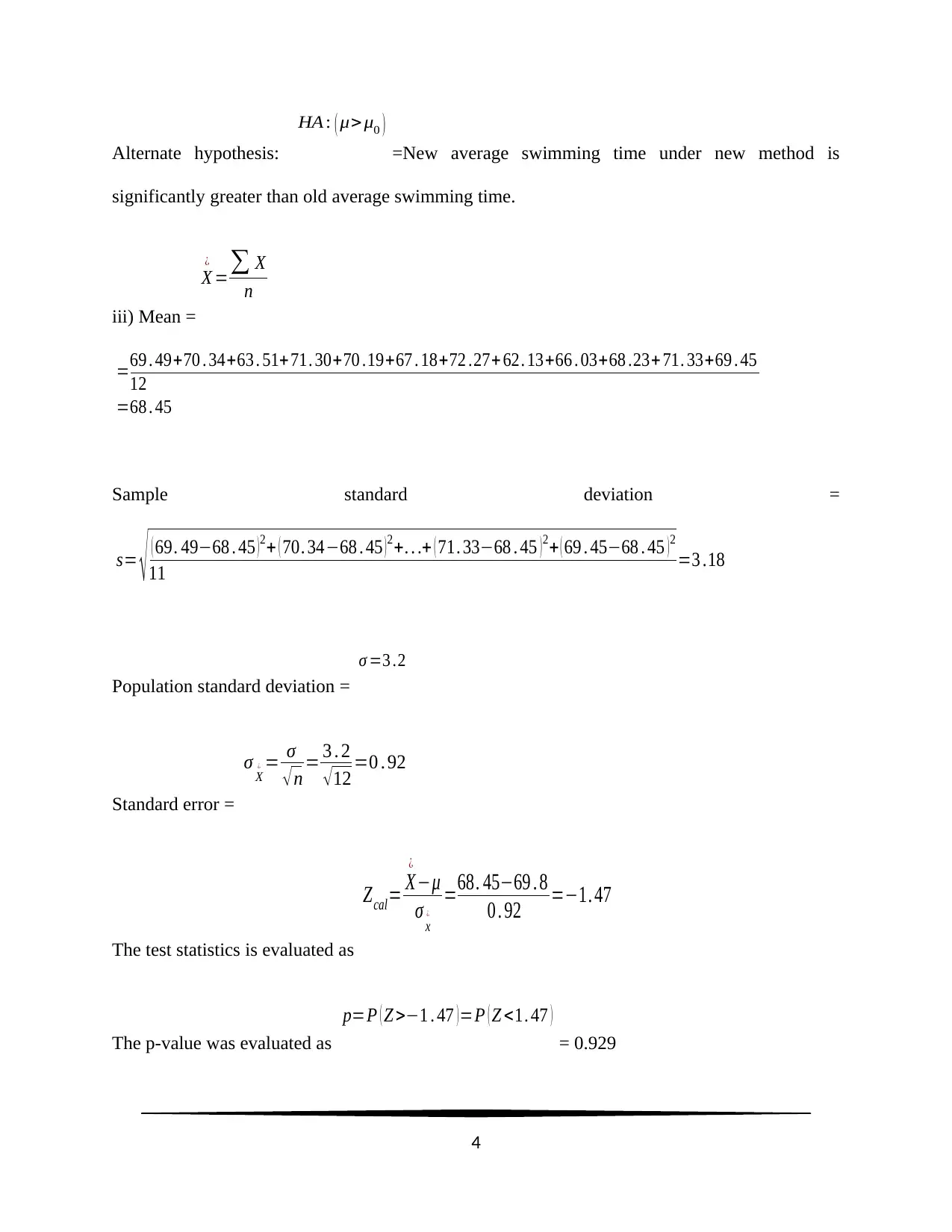
Alternate hypothesis:
HA : ( μ> μ0 )
=New average swimming time under new method is
significantly greater than old average swimming time.
iii) Mean =
X
¿
=∑ X
n
=69 . 49+70 . 34+63 . 51+ 71. 30+70 .19+67 . 18+72 .27+ 62. 13+66 . 03+68 .23+ 71. 33+69 . 45
12
=68 . 45
Sample standard deviation =
s= √ ( 69. 49−68 . 45 ) 2+ ( 70. 34−68 . 45 ) 2+. . .+ ( 71. 33−68 . 45 ) 2+ ( 69 . 45−68 . 45 ) 2
11 =3 .18
Population standard deviation =
σ =3 .2
Standard error =
σ X
¿ = σ
√ n = 3 . 2
√ 12 =0 . 92
The test statistics is evaluated as
Zcal= X
¿
−μ
σ x
¿
=68. 45−69 . 8
0 . 92 =−1. 47
The p-value was evaluated as
p=P ( Z >−1 . 47 ) =P ( Z <1. 47 )
= 0.929
4

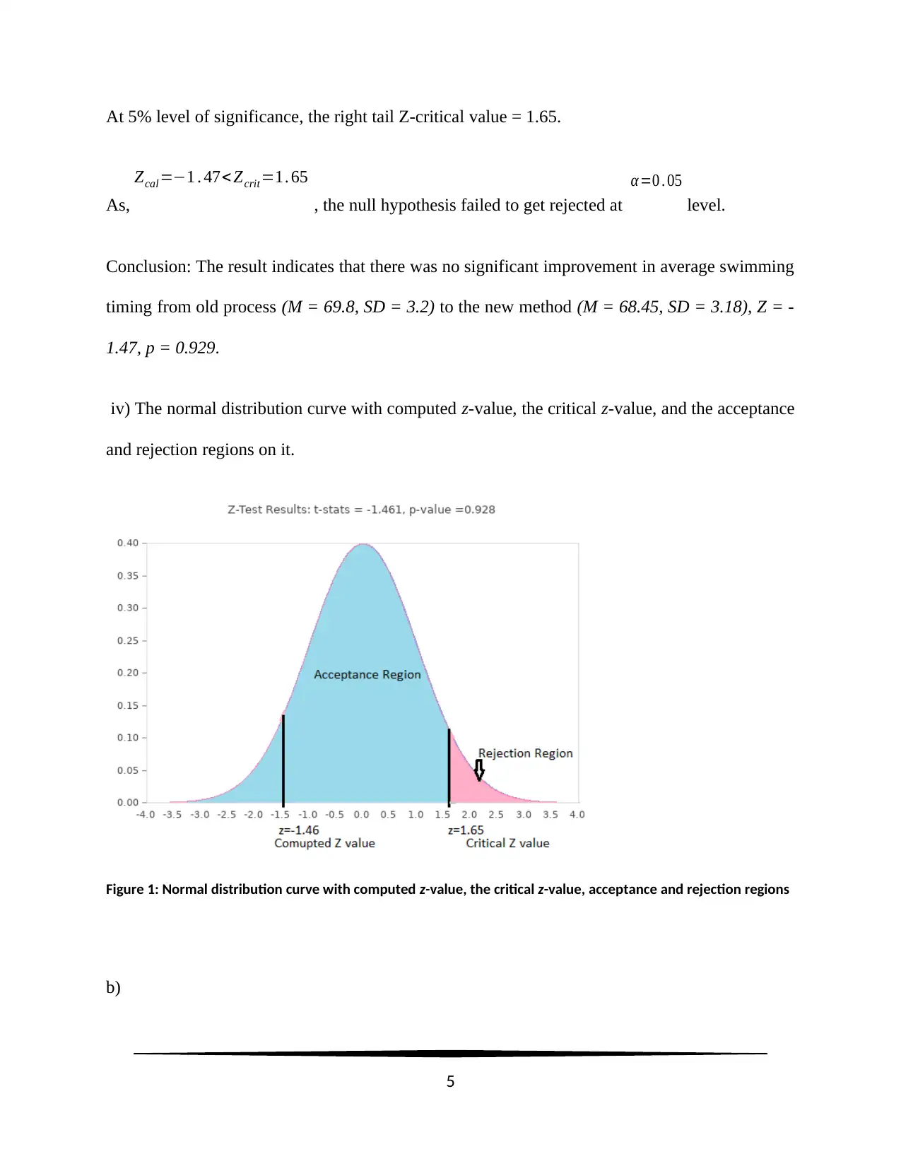
At 5% level of significance, the right tail Z-critical value = 1.65.
As,
Zcal =−1 . 47< Zcrit=1. 65
, the null hypothesis failed to get rejected at
α =0 . 05
level.
Conclusion: The result indicates that there was no significant improvement in average swimming
timing from old process (M = 69.8, SD = 3.2) to the new method (M = 68.45, SD = 3.18), Z = -
1.47, p = 0.929.
iv) The normal distribution curve with computed z-value, the critical z-value, and the acceptance
and rejection regions on it.
Figure 1: Normal distribution curve with computed z-value, the critical z-value, acceptance and rejection regions
b)
5

i) Sampling error and standard error
Difference: The difference between the population mean and sample mean is sampling error
that comes from the fact that a random sample is chosen from the population, rather than
surveying the entire population itself. This concept helps in order distinguish itself from
sampling bias. The standard error is generated when sample group is derived by dividing the
standard deviation by the square root of the number of participants.
Sampling error: The sampling error is typically the difference between the parameter of the
population and the sampling statistics, especially in size. In the statistical sense, error is
inaccuracy in estimating population parameter by the sample statistics. As population parameters
are generally not known, the sampling error function is a hypothetical perception.
Standard error: Generally, higher standard error indicates reduced sample mean as an estimate
of population parameter. This is intuitively understandable, because large sample size decreases
the standard error, and better approximates the value of the population parameter (Sedgwick,
2015).
ii) An interval scale and a ratio scale
Difference: An interval scale and a ratio scale are two variable measurement scales. Both these
scales define the attributes of the variables quantitatively. The primary difference between is
that, while interval scales can measure below absolute zero, ratio scales have a true zero value.
For example temperature is an interval score which can be below 0 degree Celsius (-10 or -20).
Again, height (ratio scale) is always above zero and cannot be never zero.
6

Interval scale: The interval scale is a numerical measurement scale, where the variables are
measured in actual manner, but, not as a relative manner. So, the presence of zero is subjective.
Hence, difference between two variables on this scale is an actual difference.
Ratio scale: This scale measures quantitative variable in nature. This allows comparing the
intervals or differences. Ratio scale possesses a zero point, which is a unique feature of ratio
scale.
iii) A statistic and a parameter
Difference: A parameter describes a summary of the characteristics of the specified population,
whereas, the statistic summarizes a small group of population or a sample.
Statistic: A statistic is obtained from the analysis of a sample. Generally, it is a descriptive
statistical measure of sample observation. As sample is a segment of the population with almost
all the characteristics of population, statistic estimates a particular population parameter.
Parameter: Parameters are a set of characteristics of the population. Here population is
considered to contain all available observations under consideration with common
characteristics. A parameter indicates the true value as every member of the population is
surveyed.
Question 9
a) Null hypothesis:
H 0: ( ρ=0 )
: there is no correlation between academic performance and
family closeness for secondary 3 students.
7

Alternate hypothesis:
HA : ( ρ>0 )
: there is a significant positive correlation between academic
performance and family closeness for secondary 3 students.
The level of significance for this test is considered as
α =0 . 05
Degrees of freedom for this test =
df =500−2=498
Test statistics,
r=0. 567
, p < 0.05 (From SPSS output)
Conclusion: As p-value is less than level of significance the null hypothesis is rejected at 5%
level. Hence, it was concluded that there is a significant positive correlation (
r ( 498 ) =0 .567
,
p<0 . 05
) between academic performance and family closeness for secondary 3 students.
b) Academic performance was measured as ratio scale variable (GPA) and family closeness was
also measured as ratio scale (continuous) variable. Pearson correlation coefficient is used to find
linear association between two interval or ratio level variables, which should be normally
distributed. Spearman rank correlation does not assume anything about the distribution of the
variables and is a non-parametric test to find monotonic association between two continuous or
ordinal variables based on the ranked values. In the present scenario, Pearson’s correlation is best
test for measuring the correlation compared to Spearman rank correlation (Hauke, & Kossowski,
2011).
8

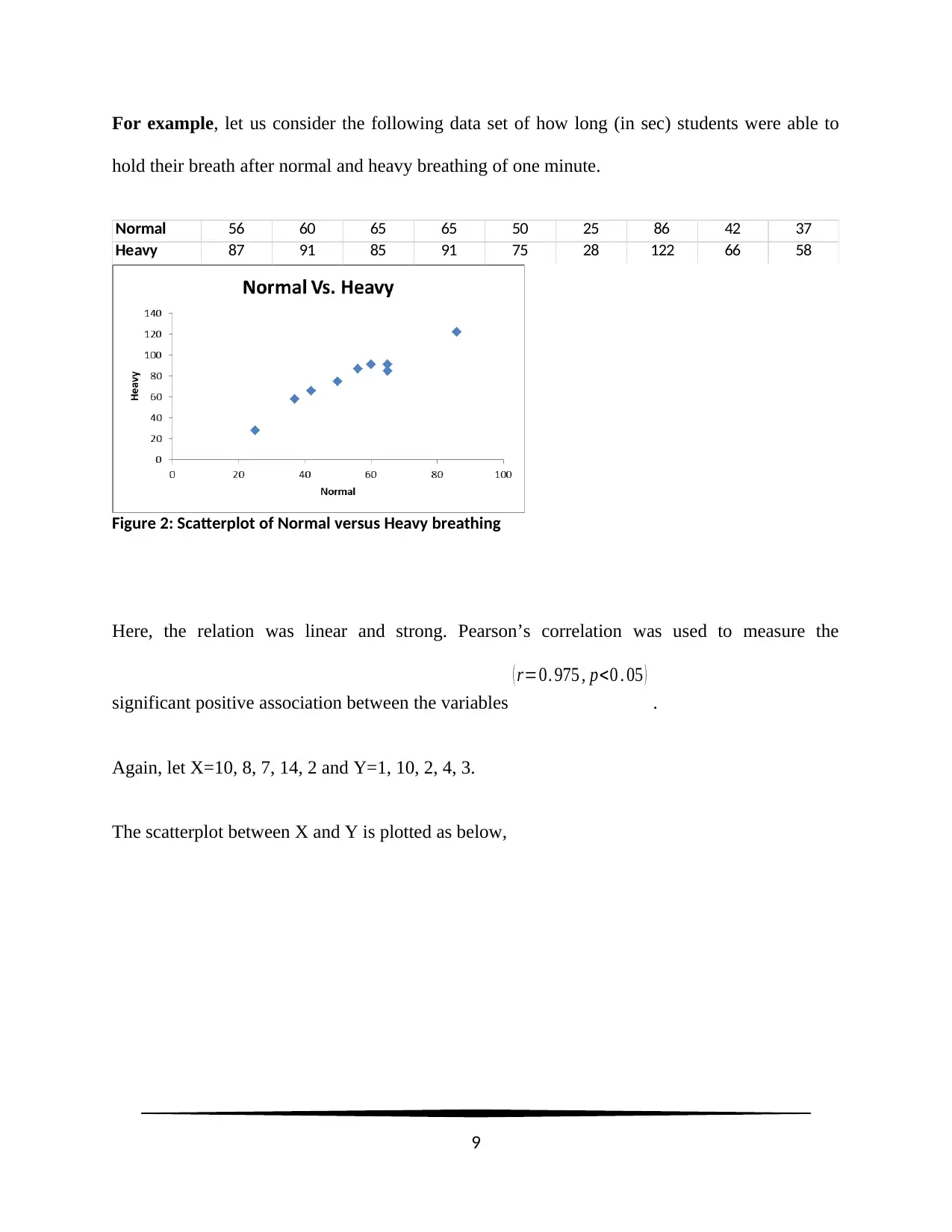
For example, let us consider the following data set of how long (in sec) students were able to
hold their breath after normal and heavy breathing of one minute.
Normal 56 60 65 65 50 25 86 42 37
Heavy 87 91 85 91 75 28 122 66 58
Figure 2: Scatterplot of Normal versus Heavy breathing
Here, the relation was linear and strong. Pearson’s correlation was used to measure the
significant positive association between the variables
( r=0. 975 , p<0 . 05 )
.
Again, let X=10, 8, 7, 14, 2 and Y=1, 10, 2, 4, 3.
The scatterplot between X and Y is plotted as below,
9

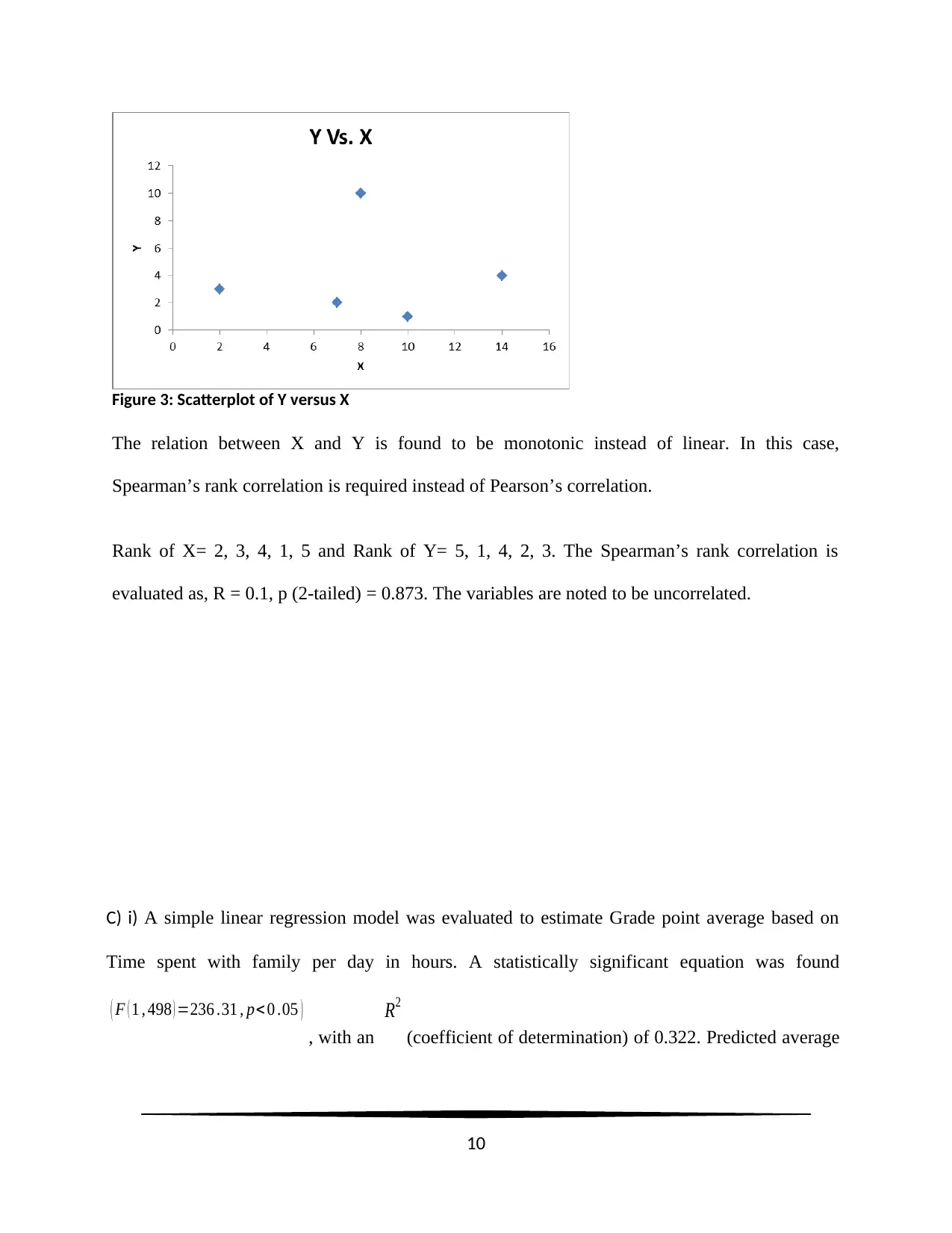
Figure 3: Scatterplot of Y versus X
The relation between X and Y is found to be monotonic instead of linear. In this case,
Spearman’s rank correlation is required instead of Pearson’s correlation.
Rank of X= 2, 3, 4, 1, 5 and Rank of Y= 5, 1, 4, 2, 3. The Spearman’s rank correlation is
evaluated as, R = 0.1, p (2-tailed) = 0.873. The variables are noted to be uncorrelated.
C) i) A simple linear regression model was evaluated to estimate Grade point average based on
Time spent with family per day in hours. A statistically significant equation was found
( F ( 1 , 498 ) =236 .31 , p< 0 .05 )
, with an
R2
(coefficient of determination) of 0.322. Predicted average
10

grade point is
2. 42+ 0. 30∗Time spent with family per day
, where the time spent in a day is
measured in hours is a significant predictor
( t =15 .37 , p<0 . 05 )
. Average grade point increased by
0.30 for one hour of extra time spent with the family in a day.
ii) The regression equation is estimated as,
Grade point average =2. 42+0 . 30∗Time spent with family per day
Student A spends an average 1.5 hours per day with family members.
His/her Grade point average =2. 42+0 . 30∗1. 5=2 . 87 hours
Student B spends an average 4.5 hours per day with family members.
His/her Grade point average =2. 42+0 . 30∗4 . 5=3 . 77 hours
Increase in time spent per day with family members, increases average grade point of a student.
Extra one hour of time spent per day with family increases average grade point by almost 0.30
units (Schielzeth, 2010).
Question 10
a) i) Null hypothesis:
H 0: ( μ1=μ2 )
: Average anger Propensity scores are equal for males and
females aged between 21 and 55 years.
11

Alternate hypothesis:
H 0: ( μ1≠μ2 )
: Average anger Propensity scores are significantly different
for males and females aged between 21 and 55 years.
ii) The independent samples t-test indicated that average anger Propensity scores for males
( M=3 . 91, SD=1. 4 , N =114 ) was considerably higher than average anger Propensity scores of
females ( M =3 . 47 , SD=1. 15 , N=136 ) , t (248 )=2 . 76 , p< 0. 05 , two-tailed. The difference of 0.44
scale scores was large ( scale range :1 to 10 ) , and the 95% confidence interval (α =.05) around
difference between average anger Propensity scores of males and females was relatively accurate
( 0 .13 , 0 . 76 ) .
iii) Assumption on the equality of variances in the above independent samples t-test was tested
using Levene’s test of equality of variances (Nordstokke, & Zumbo, 2010).
Null hypothesis:
H 0: ( σ1
2=σ2
2 )
: Variances of anger Propensity scores are equal for males and
females aged between 21 and 55 years.
Alternate hypothesis
HA : ( σ 1
2≠σ2
2 )
: Variances of anger Propensity scores are not equal for males
and females aged between 21 and 55 years.
At α =.05, the test statistics was evaluated as ( F ( 1 , 248 ) =0 . 80 , p=0 . 37 ) .
The p-value = 0.37 > At α =.05 implied that there is not enough statistical evidence to reject the
null hypothesis.
12