Numeracy and Data Analysis: Data Analysis and Forecasting

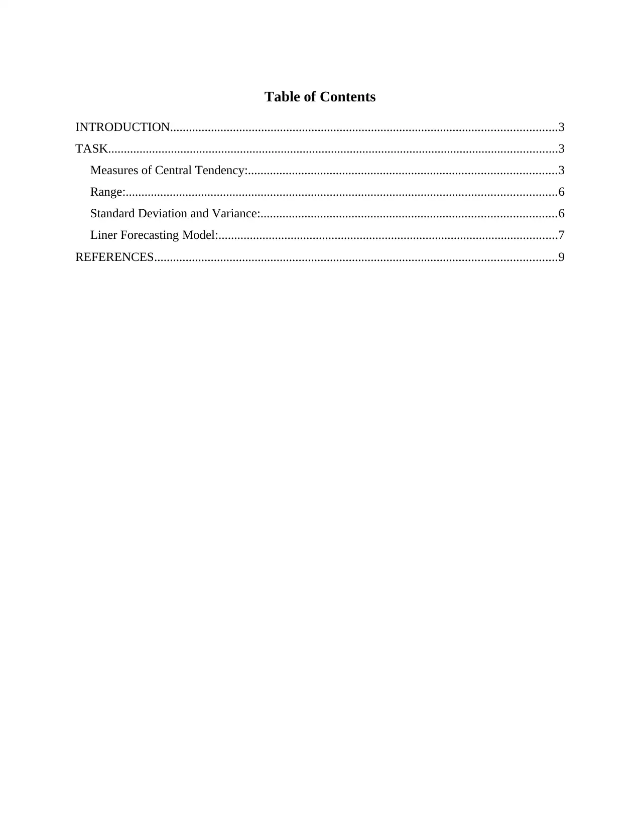
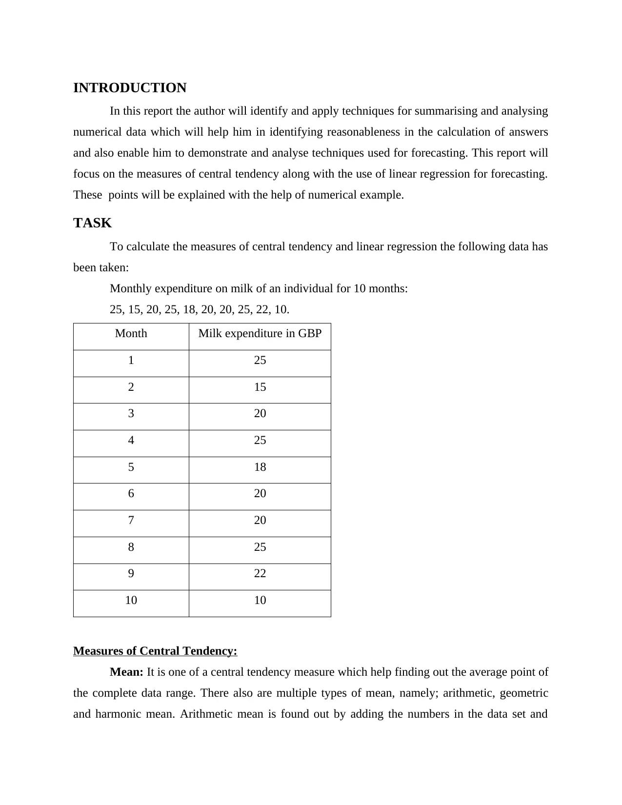
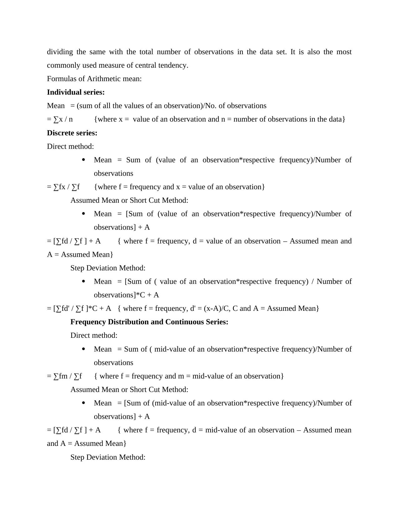
This report provides a detailed exploration of data analysis and forecasting techniques. It begins with an introduction outlining the objectives and scope of the report, followed by a task section detailing the calculation of measures of central tendency, including mean, median, and mode, using a numerical example of monthly milk expenditure. The report then delves into the calculation of range, standard deviation, and variance to assess data dispersion. Furthermore, it explains and applies linear regression for forecasting, including the calculation of slope and constant, to predict future values. The report concludes with a reference list of relevant sources used in the analysis. This report is a comprehensive guide to data analysis and forecasting, providing practical examples and calculations to aid in understanding the key concepts.

Data Analysis and
Forecasting

Table of Contents
INTRODUCTION...........................................................................................................................3
TASK...............................................................................................................................................3
Measures of Central Tendency:..................................................................................................3
Range:.........................................................................................................................................6
Standard Deviation and Variance:..............................................................................................6
Liner Forecasting Model:............................................................................................................7
REFERENCES................................................................................................................................9

INTRODUCTION
In this report the author will identify and apply techniques for summarising and analysing
numerical data which will help him in identifying reasonableness in the calculation of answers
and also enable him to demonstrate and analyse techniques used for forecasting. This report will
focus on the measures of central tendency along with the use of linear regression for forecasting.
These points will be explained with the help of numerical example.
TASK
To calculate the measures of central tendency and linear regression the following data has
been taken:
Monthly expenditure on milk of an individual for 10 months:
25, 15, 20, 25, 18, 20, 20, 25, 22, 10.
Month Milk expenditure in GBP
1 25
2 15
3 20
4 25
5 18
6 20
7 20
8 25
9 22
10 10
Measures of Central Tendency:
Mean: It is one of a central tendency measure which help finding out the average point of
the complete data range. There also are multiple types of mean, namely; arithmetic, geometric
and harmonic mean. Arithmetic mean is found out by adding the numbers in the data set and

dividing the same with the total number of observations in the data set. It is also the most
commonly used measure of central tendency.
Formulas of Arithmetic mean:
Individual series:
Mean = (sum of all the values of an observation)/No. of observations
= ∑x / n {where x = value of an observation and n = number of observations in the data}
Discrete series:
Direct method:
 Mean = Sum of (value of an observation*respective frequency)/Number of
observations
= ∑fx / ∑f {where f = frequency and x = value of an observation}
Assumed Mean or Short Cut Method:
 Mean = [Sum of (value of an observation*respective frequency)/Number of
observations] + A
= [∑fd / ∑f ] + A { where f = frequency, d = value of an observation – Assumed mean and
A = Assumed Mean}
Step Deviation Method:
 Mean = [Sum of ( value of an observation*respective frequency) / Number of
observations]*C + A
= [∑fd' / ∑f ]*C + A { where f = frequency, d' = (x-A)/C, C and A = Assumed Mean}
Frequency Distribution and Continuous Series:
Direct method:
 Mean = Sum of ( mid-value of an observation*respective frequency)/Number of
observations
= ∑fm / ∑f { where f = frequency and m = mid-value of an observation}
Assumed Mean or Short Cut Method:
 Mean = [Sum of (mid-value of an observation*respective frequency)/Number of
observations] + A
= [∑fd / ∑f ] + A { where f = frequency, d = mid-value of an observation – Assumed mean
and A = Assumed Mean}
Step Deviation Method:

 Mean = [Sum of (mid-value of an observation*respective frequency)/Number of
observations]* C + A
= [∑fd' / ∑f ]*C + A { where f = frequency, d' = (m-A)/C, C and A = Assumed Mean}
Calculation of mean from the above data:
Mean = ∑x / n
= (25+15+20+25+18+20+20+25+22+10) / 10
= 200/10
= 20
20 GBP is the Mean or average per month expenditure on milk.
Median: Median shows the value of a statistically discrete data series. In other words,
median divides the complete data set into two parts with equal number of values and one of the
part has values greater than median and the other has the value lower than the median. To
calculate median the data is needed to be arranged in ascending or descending order.
Formulas of Median:
1. Individual series:
◦ when the number of observations are odd:
M= Size of [(N+1)/2]th term { where n = number of observations}
◦ when the number of observations are even:
M = [Size of [(N/2)]th term + Size of [(N/2)+1]th term]/2 { where n = number of observations}
2. Discrete series:
M = Size of [(N+1)/2]th term { where n = ∑f}
3. Frequency Distribution and Continuous Series
M = l/2 + h/f [ N/2 – C.F. ] { where l= lower limit of the median class, h = size of the median
class, f = frequency of the median class, N = sum of frequencies and C.F. = cumulative
frequency of the class just preceding the median class}
Calculation of Median from the following data:
25, 15, 20, 25, 18, 20, 20, 25, 22, 10
Ascending order: 10, 15, 18, 20, 20, 20, 22, 25, 25, 25
Median = [(N/2)th term+(N/2)+1th term]/2
= [(10/2)th term]+[(10/2)+1th term]/2
= [5th term+6th term]/2

= (20+20)/2
= 20
From the above calculation it can be said that 20 is the median of the above data.
Mode: Mode refers to the value which occurs the most or the maximum number of times
in the data series.
Mode = the data with the highest number of frequency
Expense Frequency
10 1
15 1
18 1
20 3
22 1
25 3
The above table shows that 20 and 25 have the highest frequency. So it can be said that
20 and 25 are the mode of data.
Range:
Range is the set of data which shows the variation form upper limit to lower limit. This is
generally used in Frequency distribution series. For example if we arrange the above data in
frequency distribution format it would be like:
Expense Frequency
10-15 1
15-20 2
20-25 7
Range of every class interval can be found out by subtracting the lower limit of the C.I.
From the upper limit. For example range of C.I. 10-15 is = 15-10 = 5.

Standard Deviation and Variance:
Standard deviation is the measure of dispersion used to calculate dispersion of the data
from its mean. It measures the variance or variability of mean due to the use of different
methods.
Standard Deviation of Individual series = √(∑x2/N)
Variance = ∑x2/N
Month Milk expenditure
in GBP
x2
1 25 625
2 15 225
3 20 400
4 25 625
5 18 324
6 20 400
7 20 400
8 25 625
9 22 484
10 10 100
Total 4208
Standard Deviation = √(4208/10)
= 20.513410248
Variance = (Standard Deviation)2
= 420.8
Liner Forecasting Model:
Linear regression is a tool which is basically used in statistics for predicting the future
values from the given past values. It uses a trend line plotted on a chart.

Slope ( m): Slope is part of regression which is used to identify the steepness in the data.
It is used to calculate the rise or fall of the data.
Constant (c) = Constant is also a part of linear regression which helps in visualizing a
constant point in the data.
Month (X) Expense (Y) X*Y X2 Y2
1 25 25 1 625
2 15 30 4 225
3 20 60 9 400
4 25 100 16 625
5 18 90 25 324
6 20 120 36 400
7 20 140 49 400
8 25 200 64 625
9 22 198 81 484
10 10 100 100 100
Total 200 1063 385 4208
Y = Mx +C
Y = Slope(x) + Constant
Constant(C): It is used to view at what value regression line crosses the Y axis. It is usually
known as Y intercept. From the above example it can seen that constant is 22.47.
Slope(M): Slope is part of regression which is used to identify the steepness or the strength in the
data. It is used to calculate the rise or fall of the data or the average rate of change . It can be seen
that rate of change in the line is negative. It show that the data is moving toward the negative
side.
Slope = n(∑xy)-(∑y)(∑x)/ n(∑x)-(∑x)
= 10(1063)-(200)(55) / 10(385)-(4208)
= 10630 – 11000 / 3850-4208

= - 370/ -358
= 1.033519553
Constant(C) = (∑y)(∑x)- (∑x)(∑xy)/n(∑x)-(∑x)
= (200)(385)- (55)(1063)/10(385)-(55)2
= 77000 – 58465/ 3850 – 3025
= 18535 / 825
= 22.466666667
Dependent Variable = Slope(x) + Constant
11 Month = 1.033519553(11) + 22.466666667
= 33.83538175
The value in the 11 month will move to 33.835
12th Month = 1.033519553(12) + 22.466666667
= 12.402234636 + 22.466666667
= 34.868901303

REFERENCES
Books and Journals
Gonçalves, C., Bessa, R.J. and Pinson, P., 2021. A critical overview of privacy-preserving
approaches for collaborative forecasting. International Journal of Forecasting. 37(1),
pp.322-342.
Kaneko, Y., 2019, November. Customer-Base Sequential Data Analysis: An Application of
Attentive Neural Networks to Sales Forecasting. In 2019 International Conference on
Data Mining Workshops (ICDMW) (pp. 349-355). IEEE.
Mehdipour Pirbazari, A. and et. al 2020. Short-Term Load Forecasting Using Smart Meter Data:
A Generalization Analysis. Processes. 8(4). p.484.
Wambura, S., Huang, J. and Li, H., 2020. Long-range forecasting in feature-evolving data
streams. Knowledge-Based Systems. 206. p.106405.