Data Analysis: Frequency Distribution, Regression, and Hypothesis Test

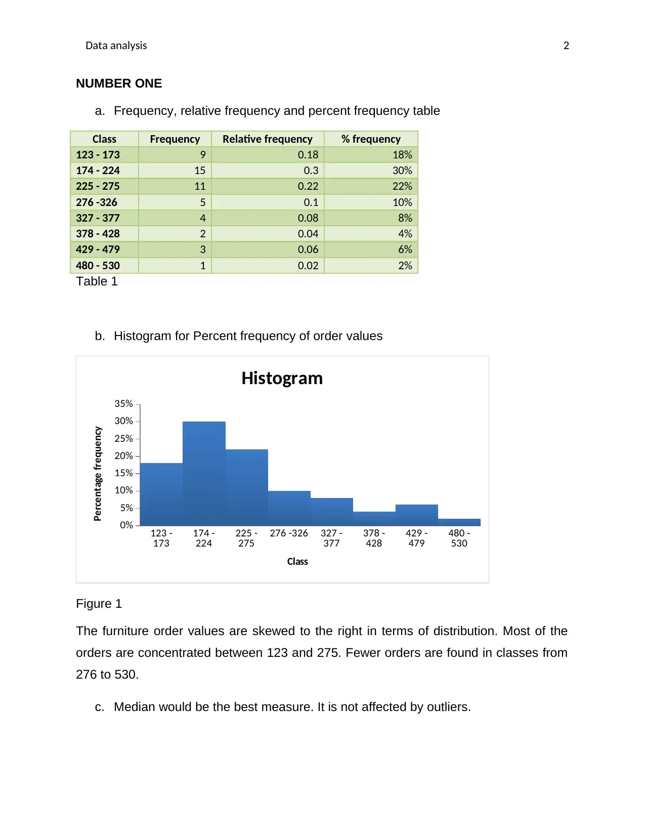
This assignment solution covers several aspects of data analysis. It includes creating a frequency distribution table, relative frequency distribution, and percent frequency distribution for furniture order values, followed by a histogram illustrating the percent frequency. The analysis reveals a right-skewed distribution. The solution also addresses regression analysis, interpreting the coefficient of determination, and conducting hypothesis tests to determine the relationship between demand and price. Furthermore, it provides a regression equation for the number of phones sold based on price and advertising spots, tests the model's significance, and interprets the gradient of coefficients. The document concludes by predicting the number of phones sold given specific price and advertising values. Desklib offers a variety of similar solved assignments and study resources for students.

Data analysis 1
Name
Instructor
Institution

Data analysis 2
NUMBER ONE
a. Frequency, relative frequency and percent frequency table
Class Frequency Relative frequency % frequency
123 - 173 9 0.18 18%
174 - 224 15 0.3 30%
225 - 275 11 0.22 22%
276 -326 5 0.1 10%
327 - 377 4 0.08 8%
378 - 428 2 0.04 4%
429 - 479 3 0.06 6%
480 - 530 1 0.02 2%
Table 1
b. Histogram for Percent frequency of order values
123 -
173 174 -
224 225 -
275 276 -326 327 -
377 378 -
428 429 -
479 480 -
530
0%
5%
10%
15%
20%
25%
30%
35%
Histogram
Class
Percentage frequency
Figure 1
The furniture order values are skewed to the right in terms of distribution. Most of the
orders are concentrated between 123 and 275. Fewer orders are found in classes from
276 to 530.
c. Median would be the best measure. It is not affected by outliers.

Data analysis 3
NUMBER TWO
a. The square of the predictor variable’s t-statistic = F (2, 47) = 74.13, reading from
F-tables, p-value tabulated is 0.000. Since 0.00 < 0.05, we do not reject the
alternative hypothesis. The conclusion is, demand and price are related.
b. Finding the Coefficient of determination
R−squared (R2 )= Regression ∑ of squares
Total ∑ of squares = 5048.818
8181.479 =0.617
The coefficient of determination is 0.617. This means the model has 61.7% predictive
capability. The independent variable explains 61.7% variation in price.
c. Coefficient of correlation
C oefficient of correlation= standard error
R2
¿ 0.248
0.617 =0.4
NUMBER THREE
Hypothesis
H0: All treatments have equal means
Versus
H1: At least one treatment has a different mean
The square of the predictor variable’s t-statistic = F (2, 23) = 16.43, reading from F-
tables, p-value tabulated is 0.000. Since 0.00 < 0.05, we do not reject the alternative
hypothesis. The conclusion is, at least one mean is different.
.

Data analysis 4
NUMBER FOUR
a. The regression equation
Number of phones sold=0.4977 ( price ) +0.4733 ( no . of advertising spots )+ 0.8051
b. Test for significance of the model
Because F (2,102) = 63.06, p < 0.001. Conclusion: the model is significant at 0.05 level
of significance
c. Test significance of coefficients
The p-value for both terms is 0.001< 0.05, it can be concluded that 1 and 2 have got
effect. The coefficient is different from zero.
d. Gradient of coefficient of X2
The slope is 0.4733. This indicates that a one unit change in independent
variable leads to a 0.4733 unit change in the number of phones sold.
e. Number of phones sold
number of phones sold=0.4977 ( 20,000 ) +0.4733 ( 10 ) +0.8051
number of phones sold=9,959.54∨9960