Data Analytics Report: Analysis of Employee Wages in Tasmania (BEA681)
VerifiedAdded on 2022/10/06
|12
|1506
|6
Report
AI Summary
This report presents a data analysis of employee information in Tasmania, focusing on the factors influencing wages. The analysis utilizes data from 150 respondents and employs various statistical techniques, including measures of central tendency to handle missing data. Categorical variables such as marriage and gender are examined, along with numerical variables like number of siblings and birth order. The study explores the relationship between education, IQ, work experience, and KW (knowledge and wisdom) with wages through scatter plots, correlation analysis, and regression analysis. Hypothesis testing is conducted to assess the average wage, and a confidence interval is calculated. The findings reveal relationships between education, IQ, KW and wages, while contradicting some newspaper criticisms. The report includes descriptive statistics, contingency tables, and probabilities to provide a comprehensive understanding of the data and the relationships between the variables.

1
Data analytics and business intelligence: Tasmania
Name:
Institution:
Data analytics and business intelligence: Tasmania
Name:
Institution:
Paraphrase This Document
Need a fresh take? Get an instant paraphrase of this document with our AI Paraphraser
2
Q1.
As evident, some variables have missing data; as a result, the study used the one of the
measures of tendency (either mean, median, or mode) to fill the missing points (Manikandan,
2011). The following table exhibits the measures of central tendency and count of variables that
have missing data. Notably, the survey incorporated 150 respondents.
wage wage hours IQ KW educ brthord meduc feduc
Mean
1075.0
6
43.9729
7
105.577
2
38.2432
4
13.7718
1
1.91911
8
11.2152
8
10.9218
8
Median 1000 40 106 39 13 1 12 11
Mode 1000 40 105 41 12 1 12 12
Count 149 148 149 148 149 136 144 128
Since, the respondents provided definite answers, it is recommendable to use the most
appearing value to fill the missing observations hence mode will be used to fill the missing
values.
Q2.
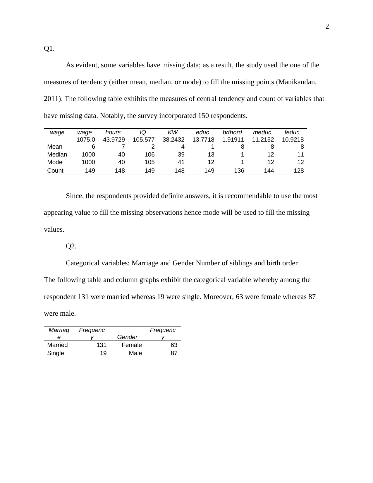
Categorical variables: Marriage and Gender Number of siblings and birth order
The following table and column graphs exhibit the categorical variable whereby among the
respondent 131 were married whereas 19 were single. Moreover, 63 were female whereas 87
were male.
Marriag
e
Frequenc
y Gender
Frequenc
y
Married 131 Female 63
Single 19 Male 87
Q1.
As evident, some variables have missing data; as a result, the study used the one of the
measures of tendency (either mean, median, or mode) to fill the missing points (Manikandan,
2011). The following table exhibits the measures of central tendency and count of variables that
have missing data. Notably, the survey incorporated 150 respondents.
wage wage hours IQ KW educ brthord meduc feduc
Mean
1075.0
6
43.9729
7
105.577
2
38.2432
4
13.7718
1
1.91911
8
11.2152
8
10.9218
8
Median 1000 40 106 39 13 1 12 11
Mode 1000 40 105 41 12 1 12 12
Count 149 148 149 148 149 136 144 128
Since, the respondents provided definite answers, it is recommendable to use the most
appearing value to fill the missing observations hence mode will be used to fill the missing
values.
Q2.
Categorical variables: Marriage and Gender Number of siblings and birth order
The following table and column graphs exhibit the categorical variable whereby among the
respondent 131 were married whereas 19 were single. Moreover, 63 were female whereas 87
were male.
Marriag
e
Frequenc
y Gender
Frequenc
y
Married 131 Female 63
Single 19 Male 87
3
Married Single
0
20
40
60
80
100
120
140
Column chart for Marriage
Female Male
0
10
20
30
40
50
60
70
80
90
100
Column chart of Gender
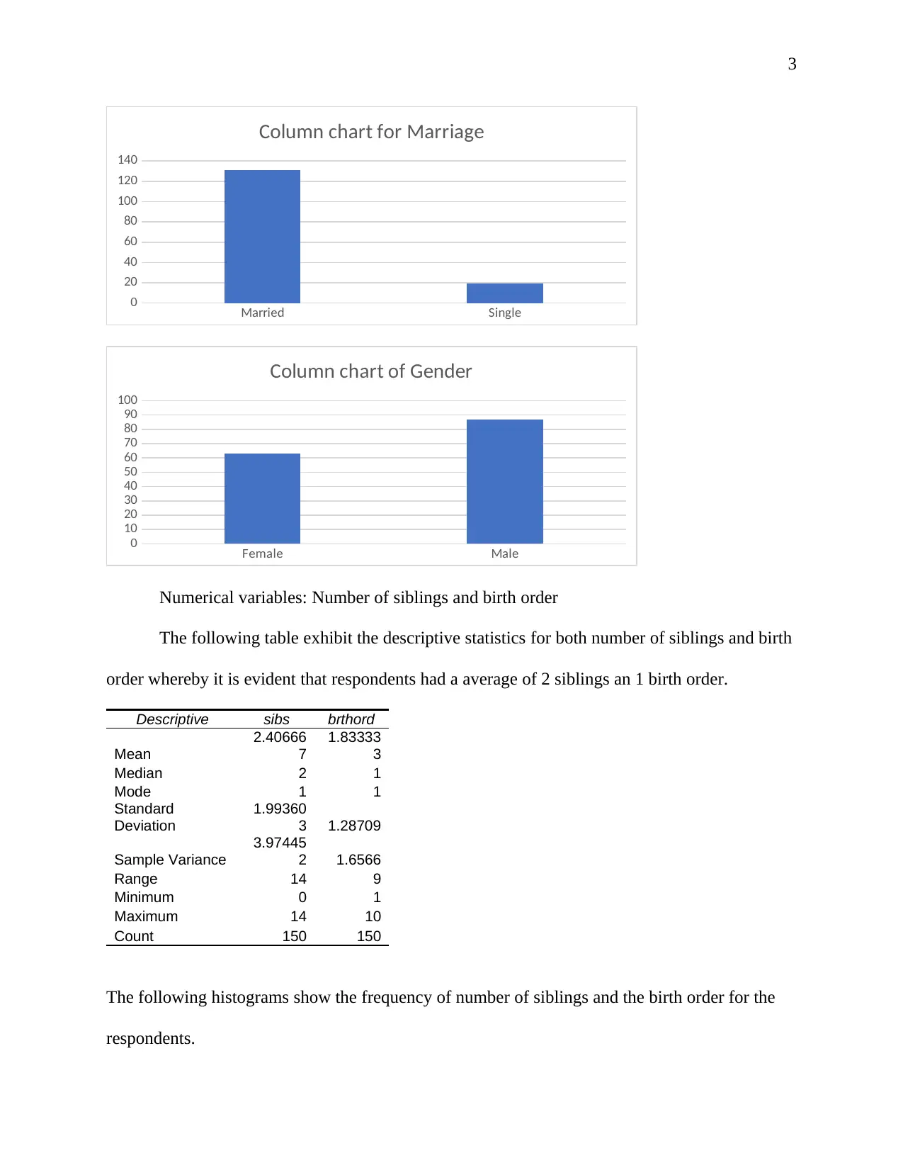
Numerical variables: Number of siblings and birth order
The following table exhibit the descriptive statistics for both number of siblings and birth
order whereby it is evident that respondents had a average of 2 siblings an 1 birth order.
Descriptive sibs brthord
Mean
2.40666
7
1.83333
3
Median 2 1
Mode 1 1
Standard
Deviation
1.99360
3 1.28709
Sample Variance
3.97445
2 1.6566
Range 14 9
Minimum 0 1
Maximum 14 10
Count 150 150
The following histograms show the frequency of number of siblings and the birth order for the
respondents.
Married Single
0
20
40
60
80
100
120
140
Column chart for Marriage
Female Male
0
10
20
30
40
50
60
70
80
90
100
Column chart of Gender
Numerical variables: Number of siblings and birth order
The following table exhibit the descriptive statistics for both number of siblings and birth
order whereby it is evident that respondents had a average of 2 siblings an 1 birth order.
Descriptive sibs brthord
Mean
2.40666
7
1.83333
3
Median 2 1
Mode 1 1
Standard
Deviation
1.99360
3 1.28709
Sample Variance
3.97445
2 1.6566
Range 14 9
Minimum 0 1
Maximum 14 10
Count 150 150
The following histograms show the frequency of number of siblings and the birth order for the
respondents.
⊘ This is a preview!⊘
Do you want full access?
Subscribe today to unlock all pages.
Trusted by 1+ million students worldwide
4
1-3 4-6 7-9 10-12 13-15
0
20
40
60
80
100
120
140
Histogram for birth order
1-3 4-6 7-9 10-12
0
20
40
60
80
100
120
140
160
Histogram for number of siblings
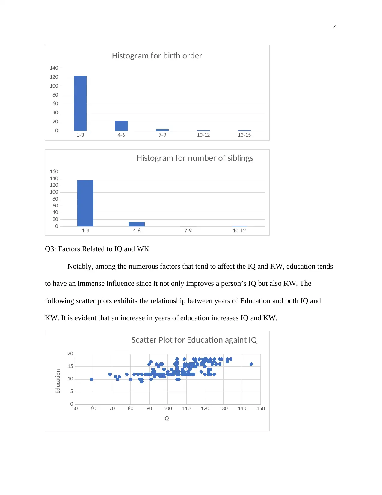
Q3: Factors Related to IQ and WK
Notably, among the numerous factors that tend to affect the IQ and KW, education tends
to have an immense influence since it not only improves a person’s IQ but also KW. The
following scatter plots exhibits the relationship between years of Education and both IQ and
KW. It is evident that an increase in years of education increases IQ and KW.
50 60 70 80 90 100 110 120 130 140 150
0
5
10
15
20
Scatter Plot for Education againt IQ
IQ
Education
1-3 4-6 7-9 10-12 13-15
0
20
40
60
80
100
120
140
Histogram for birth order
1-3 4-6 7-9 10-12
0
20
40
60
80
100
120
140
160
Histogram for number of siblings
Q3: Factors Related to IQ and WK
Notably, among the numerous factors that tend to affect the IQ and KW, education tends
to have an immense influence since it not only improves a person’s IQ but also KW. The
following scatter plots exhibits the relationship between years of Education and both IQ and
KW. It is evident that an increase in years of education increases IQ and KW.
50 60 70 80 90 100 110 120 130 140 150
0
5
10
15
20
Scatter Plot for Education againt IQ
IQ
Education
Paraphrase This Document
Need a fresh take? Get an instant paraphrase of this document with our AI Paraphraser
5
15 20 25 30 35 40 45 50 55 60
0
5
10
15
20
Education against KW
KW
Education
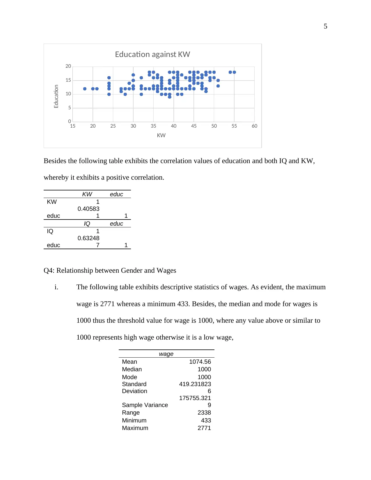
Besides the following table exhibits the correlation values of education and both IQ and KW,
whereby it exhibits a positive correlation.
KW educ
KW 1
educ
0.40583
1 1
IQ educ
IQ 1
educ
0.63248
7 1
Q4: Relationship between Gender and Wages
i. The following table exhibits descriptive statistics of wages. As evident, the maximum
wage is 2771 whereas a minimum 433. Besides, the median and mode for wages is
1000 thus the threshold value for wage is 1000, where any value above or similar to
1000 represents high wage otherwise it is a low wage,
wage
Mean 1074.56
Median 1000
Mode 1000
Standard
Deviation
419.231823
6
Sample Variance
175755.321
9
Range 2338
Minimum 433
Maximum 2771
15 20 25 30 35 40 45 50 55 60
0
5
10
15
20
Education against KW
KW
Education
Besides the following table exhibits the correlation values of education and both IQ and KW,
whereby it exhibits a positive correlation.
KW educ
KW 1
educ
0.40583
1 1
IQ educ
IQ 1
educ
0.63248
7 1
Q4: Relationship between Gender and Wages
i. The following table exhibits descriptive statistics of wages. As evident, the maximum
wage is 2771 whereas a minimum 433. Besides, the median and mode for wages is
1000 thus the threshold value for wage is 1000, where any value above or similar to
1000 represents high wage otherwise it is a low wage,
wage
Mean 1074.56
Median 1000
Mode 1000
Standard
Deviation
419.231823
6
Sample Variance
175755.321
9
Range 2338
Minimum 433
Maximum 2771
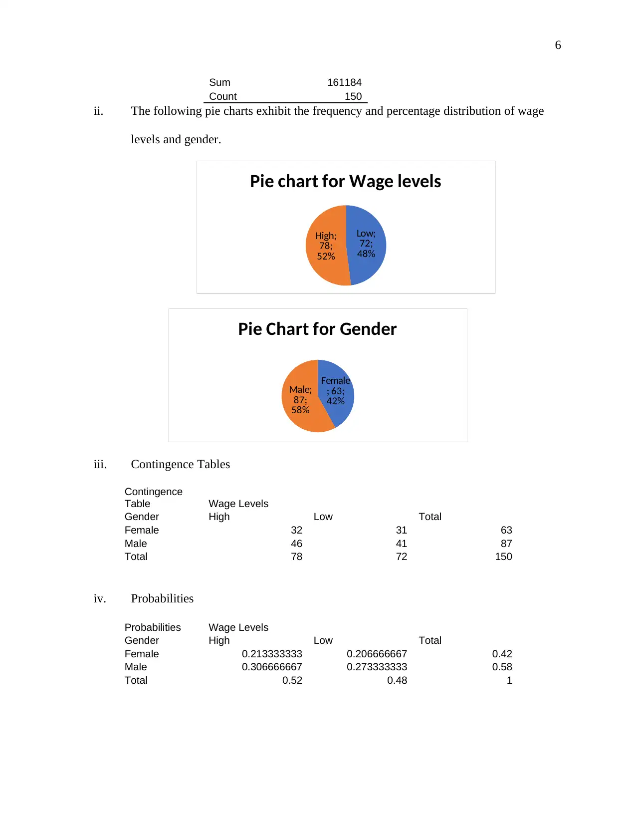
6
Sum 161184
Count 150
ii. The following pie charts exhibit the frequency and percentage distribution of wage
levels and gender.
Low;
72;
48%
High;
78;
52%
Pie chart for Wage levels
Female
; 63;
42%
Male;
87;
58%
Pie Chart for Gender
iii. Contingence Tables
Contingence
Table Wage Levels
Gender High Low Total
Female 32 31 63
Male 46 41 87
Total 78 72 150
iv. Probabilities
Probabilities Wage Levels
Gender High Low Total
Female 0.213333333 0.206666667 0.42
Male 0.306666667 0.273333333 0.58
Total 0.52 0.48 1
⊘ This is a preview!⊘
Do you want full access?
Subscribe today to unlock all pages.
Trusted by 1+ million students worldwide
7
v. The above table exhibits the probabilities of the interaction probabilities of gender
and wage levels. As evident, the probability of a female having a high wage level is
0.2133 whereas the probability of a male receiving low wage is 0.3067. Therefore, it
is evident that male tend to receive higher wages compared to female.
Q5:
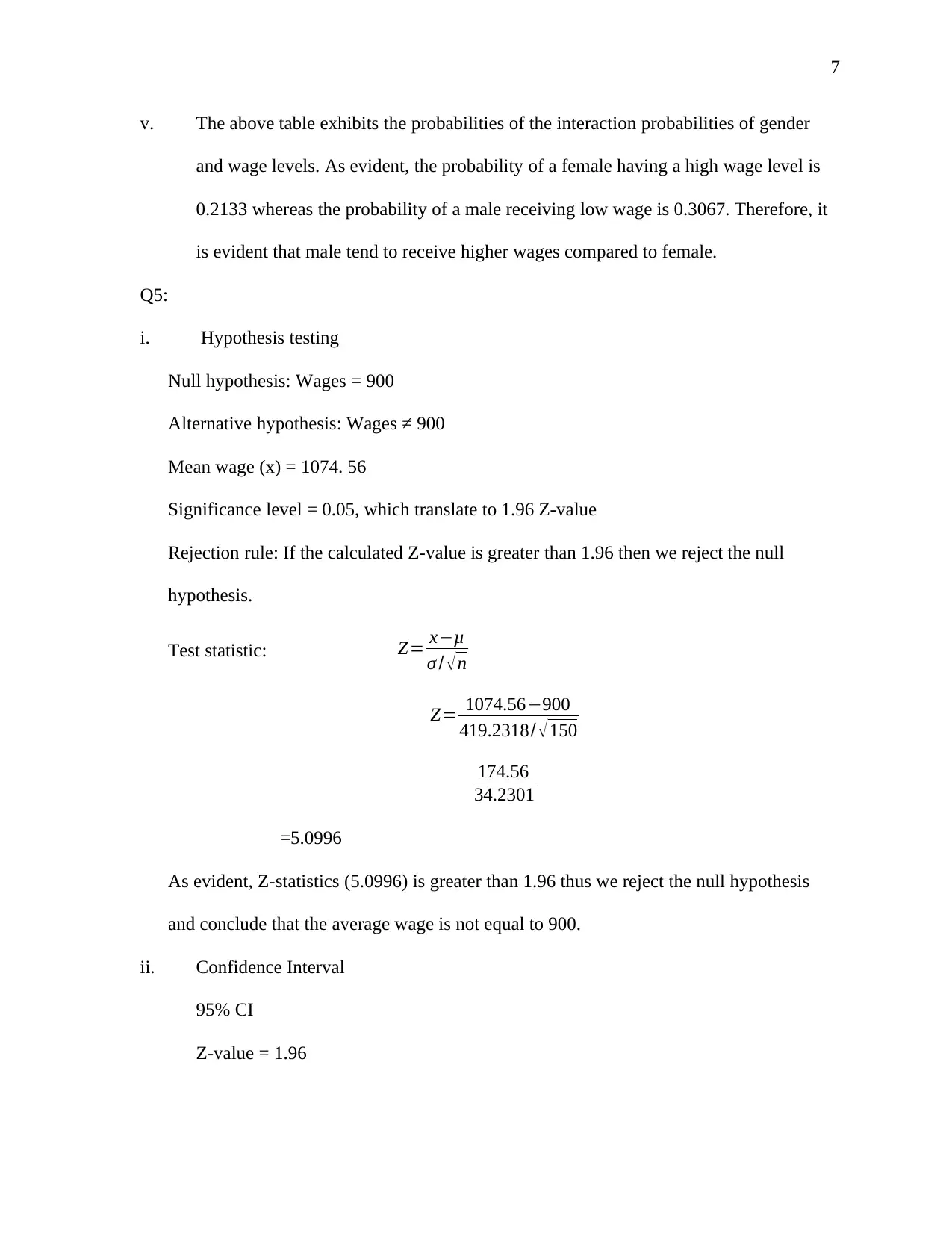
i. Hypothesis testing
Null hypothesis: Wages = 900
Alternative hypothesis: Wages ≠ 900
Mean wage (x) = 1074. 56
Significance level = 0.05, which translate to 1.96 Z-value
Rejection rule: If the calculated Z-value is greater than 1.96 then we reject the null
hypothesis.
Test statistic: Z= x−μ
σ / √ n
Z= 1074.56−900
419.2318/ √ 150
174.56
34.2301
=5.0996
As evident, Z-statistics (5.0996) is greater than 1.96 thus we reject the null hypothesis
and conclude that the average wage is not equal to 900.
ii. Confidence Interval
95% CI
Z-value = 1.96
v. The above table exhibits the probabilities of the interaction probabilities of gender
and wage levels. As evident, the probability of a female having a high wage level is
0.2133 whereas the probability of a male receiving low wage is 0.3067. Therefore, it
is evident that male tend to receive higher wages compared to female.
Q5:
i. Hypothesis testing
Null hypothesis: Wages = 900
Alternative hypothesis: Wages ≠ 900
Mean wage (x) = 1074. 56
Significance level = 0.05, which translate to 1.96 Z-value
Rejection rule: If the calculated Z-value is greater than 1.96 then we reject the null
hypothesis.
Test statistic: Z= x−μ
σ / √ n
Z= 1074.56−900
419.2318/ √ 150
174.56
34.2301
=5.0996
As evident, Z-statistics (5.0996) is greater than 1.96 thus we reject the null hypothesis
and conclude that the average wage is not equal to 900.
ii. Confidence Interval
95% CI
Z-value = 1.96
Paraphrase This Document
Need a fresh take? Get an instant paraphrase of this document with our AI Paraphraser
8
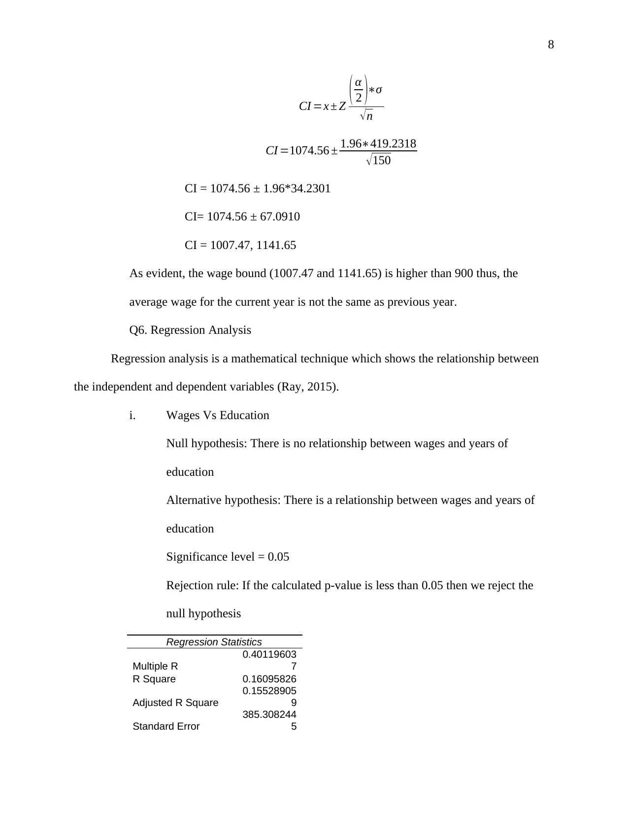
CI =x ± Z ( α
2 )∗σ
√ n
CI =1074.56 ± 1.96∗419.2318
√150
CI = 1074.56 ± 1.96*34.2301
CI= 1074.56 ± 67.0910
CI = 1007.47, 1141.65
As evident, the wage bound (1007.47 and 1141.65) is higher than 900 thus, the
average wage for the current year is not the same as previous year.
Q6. Regression Analysis
Regression analysis is a mathematical technique which shows the relationship between
the independent and dependent variables (Ray, 2015).
i. Wages Vs Education
Null hypothesis: There is no relationship between wages and years of
education
Alternative hypothesis: There is a relationship between wages and years of
education
Significance level = 0.05
Rejection rule: If the calculated p-value is less than 0.05 then we reject the
null hypothesis
Regression Statistics
Multiple R
0.40119603
7
R Square 0.16095826
Adjusted R Square
0.15528905
9
Standard Error
385.308244
5
9
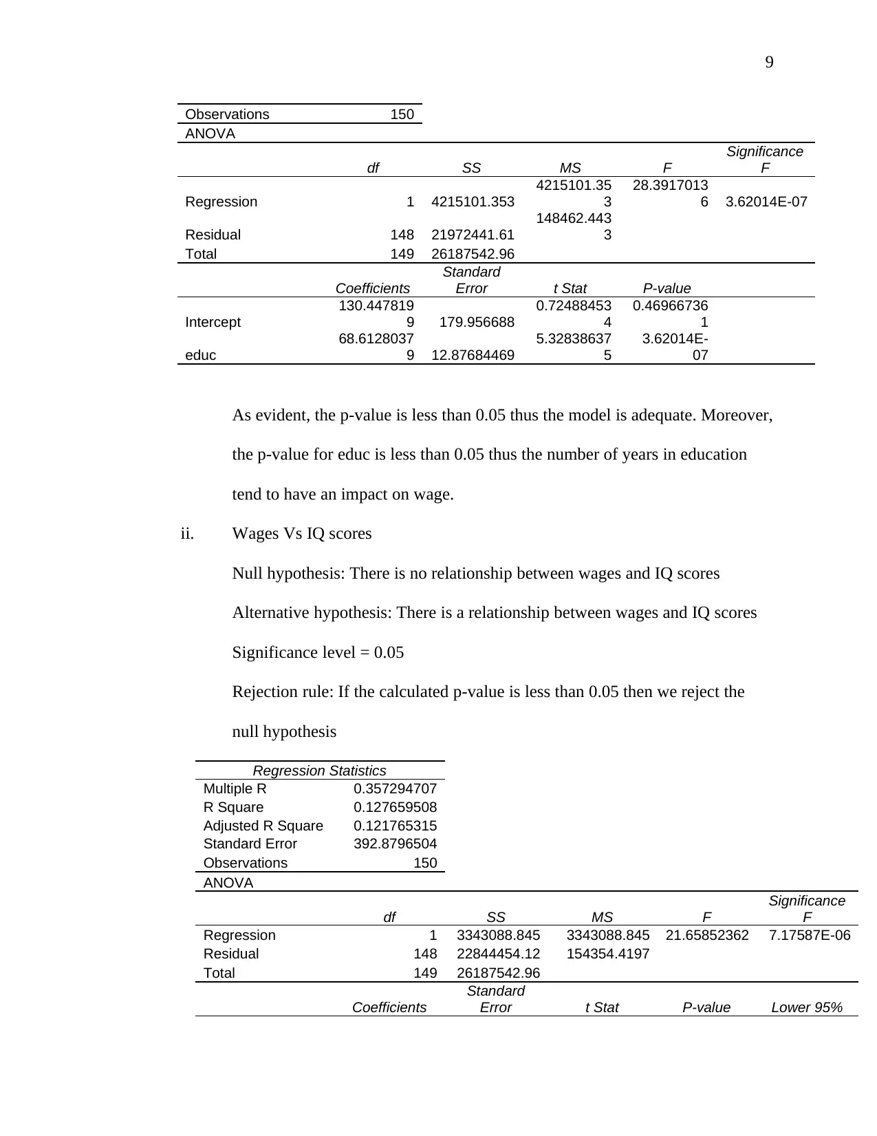
Observations 150
ANOVA
df SS MS F
Significance
F
Regression 1 4215101.353
4215101.35
3
28.3917013
6 3.62014E-07
Residual 148 21972441.61
148462.443
3
Total 149 26187542.96
Coefficients
Standard
Error t Stat P-value
Intercept
130.447819
9 179.956688
0.72488453
4
0.46966736
1
educ
68.6128037
9 12.87684469
5.32838637
5
3.62014E-
07
As evident, the p-value is less than 0.05 thus the model is adequate. Moreover,
the p-value for educ is less than 0.05 thus the number of years in education
tend to have an impact on wage.
ii. Wages Vs IQ scores
Null hypothesis: There is no relationship between wages and IQ scores
Alternative hypothesis: There is a relationship between wages and IQ scores
Significance level = 0.05
Rejection rule: If the calculated p-value is less than 0.05 then we reject the
null hypothesis
Regression Statistics
Multiple R 0.357294707
R Square 0.127659508
Adjusted R Square 0.121765315
Standard Error 392.8796504
Observations 150
ANOVA
df SS MS F
Significance
F
Regression 1 3343088.845 3343088.845 21.65852362 7.17587E-06
Residual 148 22844454.12 154354.4197
Total 149 26187542.96
Coefficients
Standard
Error t Stat P-value Lower 95%
Observations 150
ANOVA
df SS MS F
Significance
F
Regression 1 4215101.353
4215101.35
3
28.3917013
6 3.62014E-07
Residual 148 21972441.61
148462.443
3
Total 149 26187542.96
Coefficients
Standard
Error t Stat P-value
Intercept
130.447819
9 179.956688
0.72488453
4
0.46966736
1
educ
68.6128037
9 12.87684469
5.32838637
5
3.62014E-
07
As evident, the p-value is less than 0.05 thus the model is adequate. Moreover,
the p-value for educ is less than 0.05 thus the number of years in education
tend to have an impact on wage.
ii. Wages Vs IQ scores
Null hypothesis: There is no relationship between wages and IQ scores
Alternative hypothesis: There is a relationship between wages and IQ scores
Significance level = 0.05
Rejection rule: If the calculated p-value is less than 0.05 then we reject the
null hypothesis
Regression Statistics
Multiple R 0.357294707
R Square 0.127659508
Adjusted R Square 0.121765315
Standard Error 392.8796504
Observations 150
ANOVA
df SS MS F
Significance
F
Regression 1 3343088.845 3343088.845 21.65852362 7.17587E-06
Residual 148 22844454.12 154354.4197
Total 149 26187542.96
Coefficients
Standard
Error t Stat P-value Lower 95%
⊘ This is a preview!⊘
Do you want full access?
Subscribe today to unlock all pages.
Trusted by 1+ million students worldwide
10
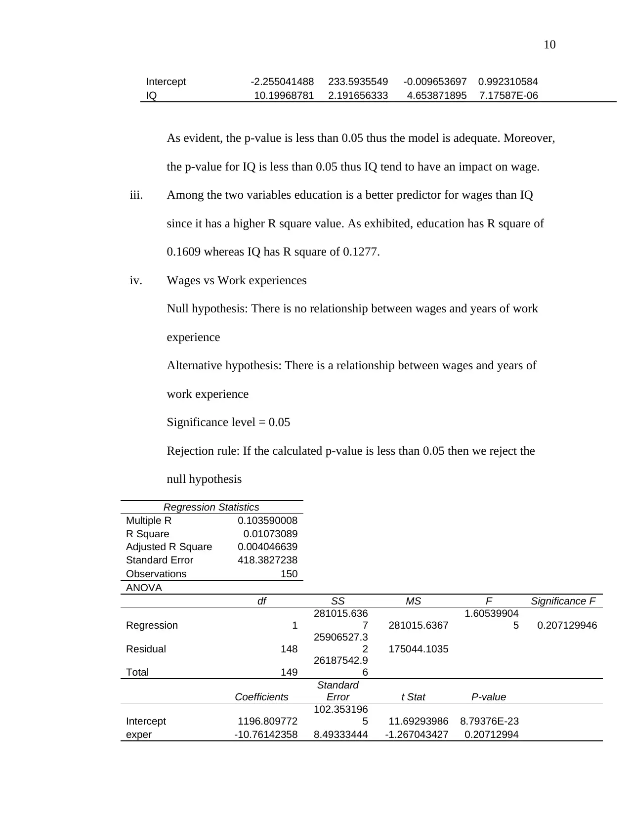
Intercept -2.255041488 233.5935549 -0.009653697 0.992310584
IQ 10.19968781 2.191656333 4.653871895 7.17587E-06
As evident, the p-value is less than 0.05 thus the model is adequate. Moreover,
the p-value for IQ is less than 0.05 thus IQ tend to have an impact on wage.
iii. Among the two variables education is a better predictor for wages than IQ
since it has a higher R square value. As exhibited, education has R square of
0.1609 whereas IQ has R square of 0.1277.
iv. Wages vs Work experiences
Null hypothesis: There is no relationship between wages and years of work
experience
Alternative hypothesis: There is a relationship between wages and years of
work experience
Significance level = 0.05
Rejection rule: If the calculated p-value is less than 0.05 then we reject the
null hypothesis
Regression Statistics
Multiple R 0.103590008
R Square 0.01073089
Adjusted R Square 0.004046639
Standard Error 418.3827238
Observations 150
ANOVA
df SS MS F Significance F
Regression 1
281015.636
7 281015.6367
1.60539904
5 0.207129946
Residual 148
25906527.3
2 175044.1035
Total 149
26187542.9
6
Coefficients
Standard
Error t Stat P-value
Intercept 1196.809772
102.353196
5 11.69293986 8.79376E-23
exper -10.76142358 8.49333444 -1.267043427 0.20712994
Paraphrase This Document
Need a fresh take? Get an instant paraphrase of this document with our AI Paraphraser
11
5 6
As evident, the p-value is greater than 0.05 thus the model is not adequate.
Moreover, the p-value for work experience is greater than 0.05 thus work
experience does not have an impact on wage.
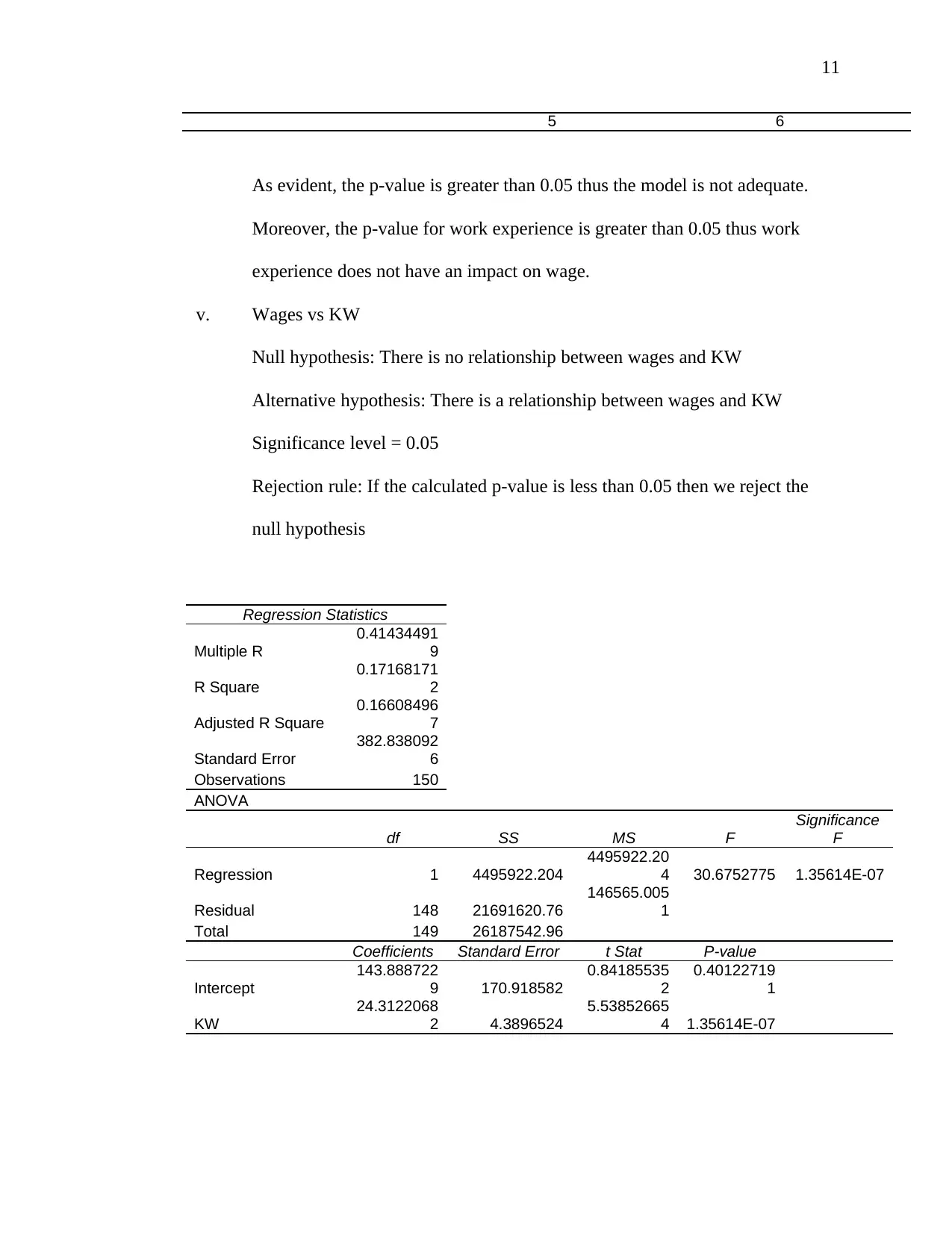
v. Wages vs KW
Null hypothesis: There is no relationship between wages and KW
Alternative hypothesis: There is a relationship between wages and KW
Significance level = 0.05
Rejection rule: If the calculated p-value is less than 0.05 then we reject the
null hypothesis
Regression Statistics
Multiple R
0.41434491
9
R Square
0.17168171
2
Adjusted R Square
0.16608496
7
Standard Error
382.838092
6
Observations 150
ANOVA
df SS MS F
Significance
F
Regression 1 4495922.204
4495922.20
4 30.6752775 1.35614E-07
Residual 148 21691620.76
146565.005
1
Total 149 26187542.96
Coefficients Standard Error t Stat P-value
Intercept
143.888722
9 170.918582
0.84185535
2
0.40122719
1
KW
24.3122068
2 4.3896524
5.53852665
4 1.35614E-07
5 6
As evident, the p-value is greater than 0.05 thus the model is not adequate.
Moreover, the p-value for work experience is greater than 0.05 thus work
experience does not have an impact on wage.
v. Wages vs KW
Null hypothesis: There is no relationship between wages and KW
Alternative hypothesis: There is a relationship between wages and KW
Significance level = 0.05
Rejection rule: If the calculated p-value is less than 0.05 then we reject the
null hypothesis
Regression Statistics
Multiple R
0.41434491
9
R Square
0.17168171
2
Adjusted R Square
0.16608496
7
Standard Error
382.838092
6
Observations 150
ANOVA
df SS MS F
Significance
F
Regression 1 4495922.204
4495922.20
4 30.6752775 1.35614E-07
Residual 148 21691620.76
146565.005
1
Total 149 26187542.96
Coefficients Standard Error t Stat P-value
Intercept
143.888722
9 170.918582
0.84185535
2
0.40122719
1
KW
24.3122068
2 4.3896524
5.53852665
4 1.35614E-07
12
As evident, the p-value is less than 0.05 thus the model is adequate. Moreover,
the p-value for KW is less than 0.05 thus KW tend to have an impact on wage.
vi. Among, the two variables KW is a better predictor since it has p-value of less
than 0.05. Moreover, it has a higher R square value of 0.1717
vii. As evident, there is no relationship between wages and work experience
whereas there is a relationship between wages and education thus the above
analysis contradicts with the newspaper’s criticism.
References
Manikandan, S. (2011). Measures of central tendency: The mean. Journal of Pharmacol &
Pharmacotherapeutics, 140-142. doi:10.4103/0976-500X.81920
Ray, S. (2015, August 14). Regression Techniques. Retrieved from Analytics Vidhya Website:
https://www.analyticsvidhya.com/blog/2015/08/comprehensive-guide-regression/
⊘ This is a preview!⊘
Do you want full access?
Subscribe today to unlock all pages.
Trusted by 1+ million students worldwide
1 out of 12
Your All-in-One AI-Powered Toolkit for Academic Success.
+13062052269
info@desklib.com
Available 24*7 on WhatsApp / Email
![[object Object]](/_next/static/media/star-bottom.7253800d.svg)
Unlock your academic potential
Copyright © 2020–2026 A2Z Services. All Rights Reserved. Developed and managed by ZUCOL.