Data Analysis Report: Analyzing Monthly Expenses Data

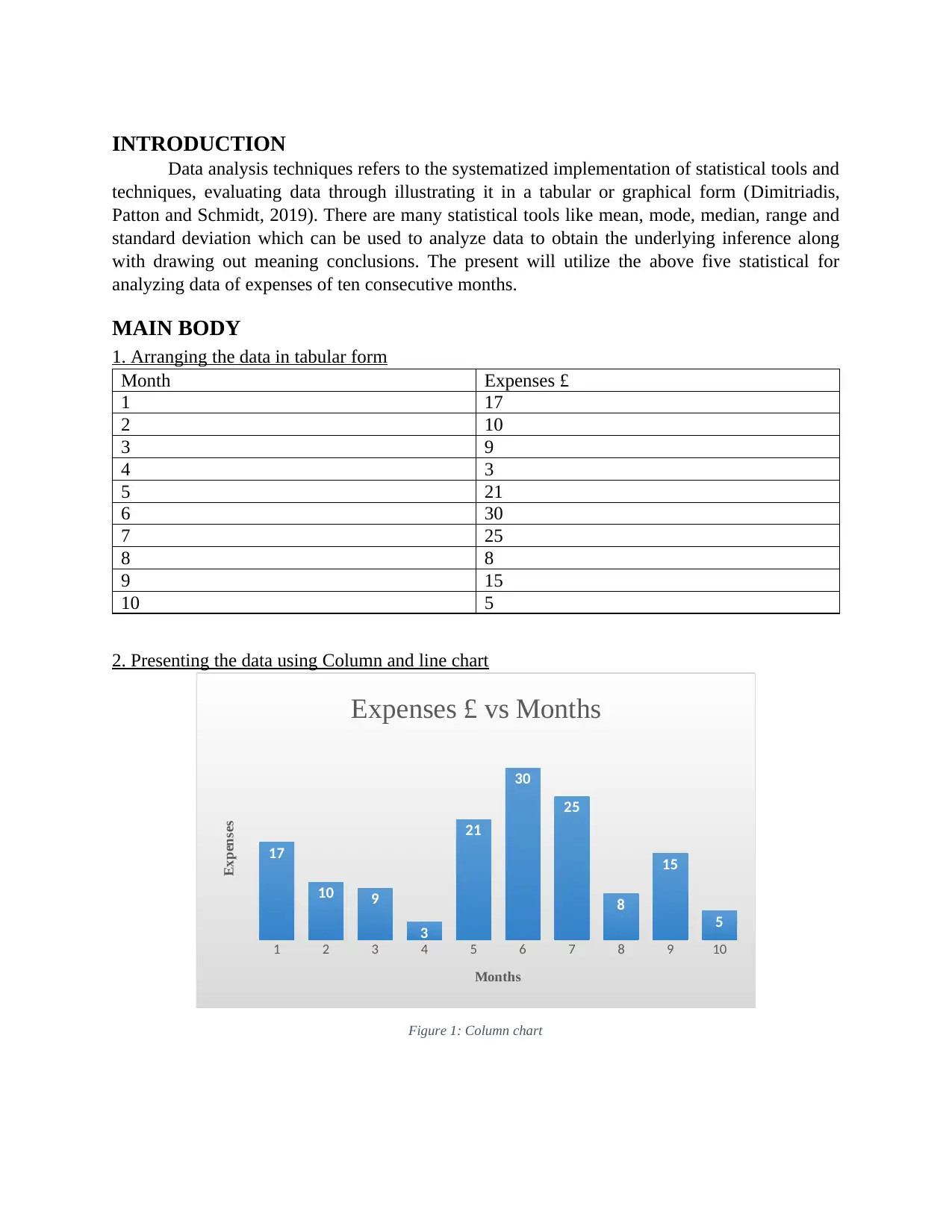
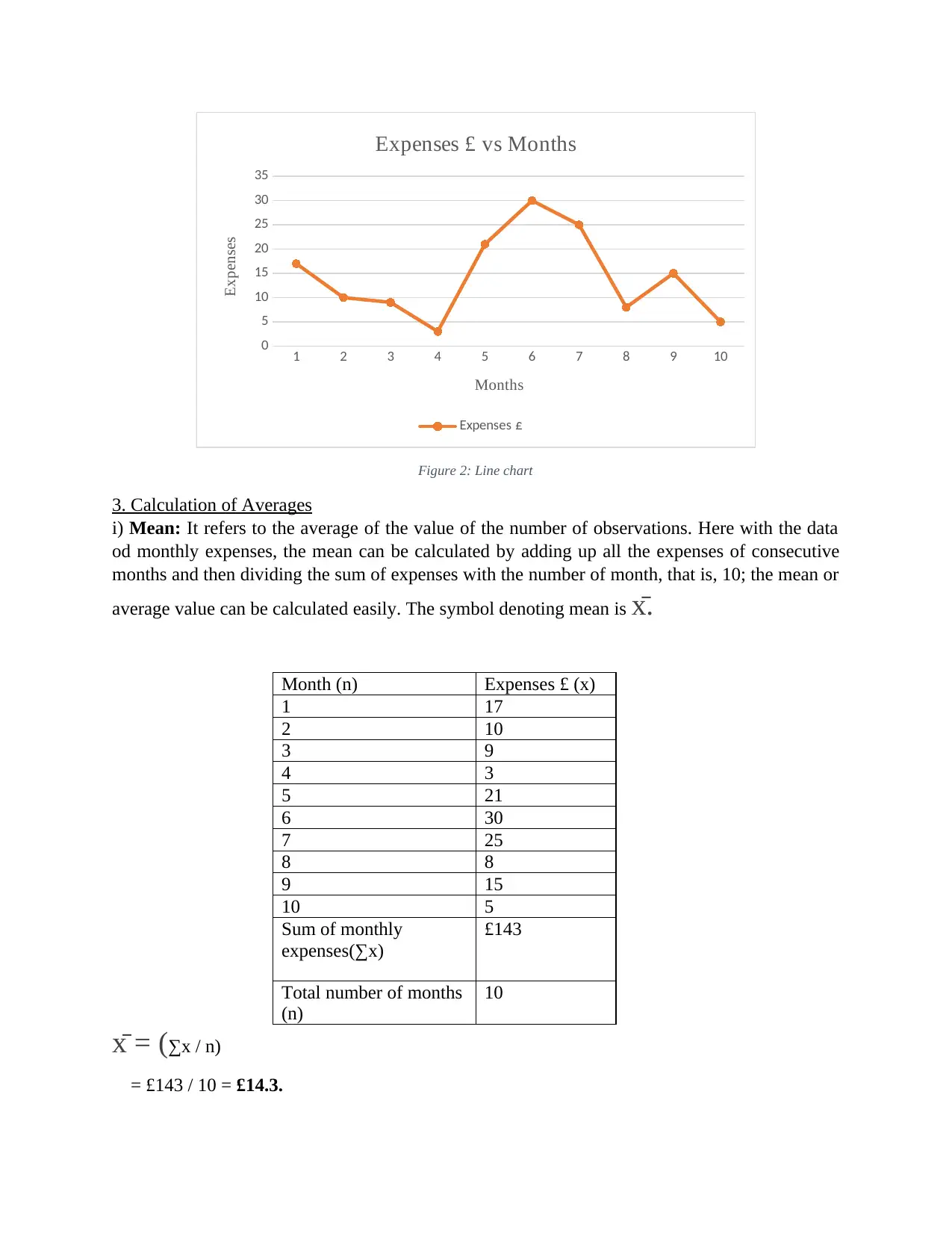
This report presents a comprehensive analysis of monthly expense data using various data analysis techniques. The analysis begins with arranging the data in a tabular format, followed by presenting the data visually using column and line charts. Averages, including mean, median, and mode, are calculated to understand the central tendencies of the data. Furthermore, the report calculates the range and standard deviation to assess data variability and dispersion. A linear forecasting model is then applied to predict future expenses for the 11th and 12th months. The report concludes with interpretations of the results obtained from each technique, providing insights into the expense patterns and future projections. The report incorporates relevant formulas and interpretations to make the analysis easily understandable.

DATA ANALYSIS
TECHNIQUES

INTRODUCTION.....................................................................................................................................3
MAIN BODY.............................................................................................................................................3
1. Arranging the data in tabular form.......................................................................................................3
2. Presenting the data using Column and line chart.................................................................................3
3. Calculation of Averages......................................................................................................................4
4. Future forecasting using linear model..................................................................................................7
CONCLUSION..........................................................................................................................................8
REFERENCES..........................................................................................................................................9

INTRODUCTION
Data analysis techniques refers to the systematized implementation of statistical tools and
techniques, evaluating data through illustrating it in a tabular or graphical form (Dimitriadis,
Patton and Schmidt, 2019). There are many statistical tools like mean, mode, median, range and
standard deviation which can be used to analyze data to obtain the underlying inference along
with drawing out meaning conclusions. The present will utilize the above five statistical for
analyzing data of expenses of ten consecutive months.
MAIN BODY
1. Arranging the data in tabular form
Month Expenses £
1 17
2 10
3 9
4 3
5 21
6 30
7 25
8 8
9 15
10 5
2. Presenting the data using Column and line chart
1 2 3 4 5 6 7 8 9 10
17
10 9
3
21
30
25
8
15
5
Expenses £ vs Months
Months
Expenses
Figure 1: Column chart

1 2 3 4 5 6 7 8 9 10
0
5
10
15
20
25
30
35
Expenses £ vs Months
Expenses £
Months
Expenses
Figure 2: Line chart
3. Calculation of Averages
i) Mean: It refers to the average of the value of the number of observations. Here with the data
od monthly expenses, the mean can be calculated by adding up all the expenses of consecutive
months and then dividing the sum of expenses with the number of month, that is, 10; the mean or
average value can be calculated easily. The symbol denoting mean is x̄.
Month (n) Expenses £ (x)
1 17
2 10
3 9
4 3
5 21
6 30
7 25
8 8
9 15
10 5
Sum of monthly
expenses(∑x)
£143
Total number of months
(n)
10
x̄ = (∑x / n)
= £143 / 10 = £14.3.

Interpretation: From the obtained value of mean, that is 14.3, it can be said that in a particular
month there are expenditure of around 14.3. It has been obtained by adding up all the expenses
of ten consecutive months, which comes out to be 143, and then divided it with 10.
ii) Median: It is also referred to as partitioned value, where the middle value of the arranged
series either in ascending or descending order is taken as median (Nastic and et.al., 2017). When
the number of observations are even, then the pair in the middle of the series is first added up and
then divided by 2, the resulting value then be taken as median value.
Step: 1- arranging the given set of data pertaining to monthly expenses of ten months in
ascending order as follows:
Month Expenses £
4 3
10 5
8 8
3 9
2 10
9 15
1 17
5 21
7 25
6 30
Step: 2 – Now, to obtain the median value, the formula, that is (n + 1) / 2, will be applied as
follows:
Total number of months = 10.
Median value = 10 + 1 / 2 = 5.5.
Median = The average of 5th and 6th items,
= 10 + 15 / 2 = £12.5.
Interpretation: The value obtained for median value indicating the position of the median here
come out to be 5.5, where the exact position cannot be determined, so the average of both the
values at 5th and 6th position will be obtained by adding them up and then dividing it by 2 to
determine the median. Here these two items of middle pair in the series are 10 and 15, and
through these value median value is determined as 12.5.
iii) Mode: In a given series of data, mode is that value of the series which has occurred most of
the time or the frequency of its occurrence is high among other frequencies of different values in
the series (Adams III, 2018). In this particular illustration of expenses of ten consecutive
months, that is, 17,10,9,3,21,30,25,8,15,5; where all the items have been appearing only for
once, so there is no modal value for this series of data.

iv) Range: It is the difference between the two extreme ends of a series, that is the greatest and
the lowest value of a series. Range is used for determining the variability in the series of data. In
the given data of monthly expenses, range can be calculated as follows:
Range = maximum value – minimum value
= 30 – 3 = 27.
Interpretation: Here range comes out be 27, which is the difference between the highest value
30 and the lowest value 3.
Standard deviation: It is a measure of dispersion in which it has been determined that how each
and every value of the series is deviating from the average or mean value of the series. Higher
value of standard deviation indicates that the data are highly spread out from the mean while the
lower value shows that the values are quite closer to the mean of the series (Guerrero and Solis-
Lemus, 2020). It has been symbolized as σ. the formula for calculating standard deviation are as
follows:
Month Expenses £
(X) (X - x̄ ) (X - x̄ )2
1 17 17 - 14.3 = 2.7 7.29
2 10 10 – 14.3 = -4.3 18.49
3 9 9 – 14.3 = -5.3 28.09
4 3 3 – 14.3 = -11.3 127.69
5 21 21 – 14.3 = 6.7 44.89
6 30 30 – 14.3 = 15.7 246.49
7 25 25 – 14.3 = 10.7 114.49
8 8 8 – 14.3 = -6.3 39.69
9 15 15 – 14.3 = 0.7 0.49
10 5 5 – 14.3 = -9.3 86.49
N = 10 ∑X = 143 ∑(X - x̄) 2 = 714.1
x̄ ∑X / N
= 143 / 10
= 14.3
= SQRT of [ ∑ (X - x̄) 2 / n]
= SQRT of [714.1 / 10]
= SQRT of [71.41] =

σ = 8.45.
Interpretation: The data of monthly expenses has a standard deviation of 8.45 from the mean of
the series.
4. Future forecasting using linear model
Linear forecasting model = y =mx + c
i) calculation of m
Step:1- calculating necessary values for the formula
Month (x) Expenses £ (y) x*y x2
1 17 17 1
2 10 20 4
3 9 27 9
4 3 12 16
5 21 105 25
6 30 180 36
7 25 175 49
8 8 64 64
9 15 135 81
10 5 50 100
∑=55 ∑=143 ∑=785 ∑=3025
m = [(n*Σxy) – (Σx*Σy)] / [(n*Σx2) – (Σx)2]
m= [(10*785)-(55*143)] / [(10*3025)-(55)2]
m=[-15] / [27225]
m= - 0.0005
ii) calculation of c
c = [Σy – (m * Σx)] / n
c=[143-(-0.0005*55)] / 10
c= 143.02 / 10
c= 14.30
iii) forecasting of 11th and 12th month
using linear forecasting model, that is, y=mx + c
for 11th month expenses would be as follows:
x = 11, mx = -0.0005*11, c=14.30
y= -0.0005(11) + 14.30

y = 14.29
So, in eleventh month the expenses would be 14.29 as forecasted.
For 12th month expenses, x = 12, mx = -0.0005*12, c = 14.30
y = -0.0005(12) + 14.30
y = 14.294.
So, in 12th month the expenses would be 14.294 as forecasted.
CONCLUSION
From the above report prepared on various data analysis techniques, it can be concluded
that how different statistical techniques shows different results and accordingly they are
interpreted differently.

REFERENCES
Books and Journals
Nastic, S., and et.al., 2017. A serverless real-time data analytics platform for edge
computing. IEEE Internet Computing, 21(4), pp.64-71.
Dimitriadis, T., Patton, A. J. and Schmidt, P., 2019. Testing forecast rationality for measures of
central tendency. arXiv preprint arXiv:1910.12545.
Adams III, T. E., 2018. The use of central tendency measures from an operational short lead-time
hydrologic ensemble forecast system for real-time forecasts (Doctoral dissertation,
Virginia Tech).
Guerrero, V. M. and Solis-Lemus, C., 2020. A generalized measure of dispersion. Statistics &
Probability Letters, 164. p.108806.