Statistics Assignment: Data Analysis & Interpretation, UTS Autumn 2019

This document provides a detailed solution to a statistics assignment, utilizing both Minitab and SPSS for data analysis and interpretation. The assignment covers various statistical concepts, including descriptive statistics, chi-square tests, and regression modeling. Minitab is used to analyze the relationship between smoking habits, exercise frequency, and pulse rates, while SPSS is employed to assess the correlation between weight and height, evaluate the normality of distributions, and calculate predicted values using regression models. The solution includes statistical and graphical evidence to support the findings, offering a comprehensive understanding of the data and statistical design principles. This student-contributed assignment is available on Desklib, a platform offering a wealth of study resources for students.

Statistics
Student Name:
Instructor Name:
Course Number:
3 April 2019

QUESTION 1. Working with Minitab
(a) What percentage of
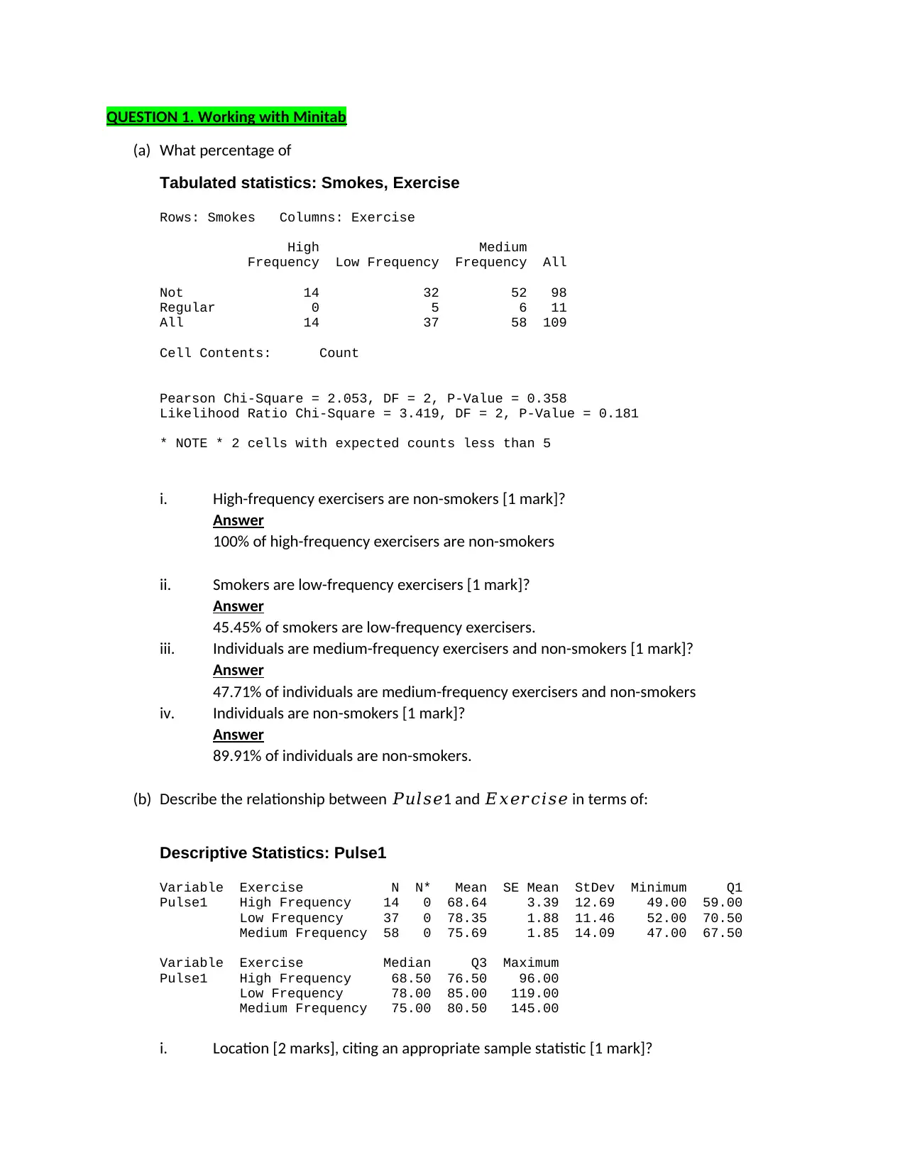
Tabulated statistics: Smokes, Exercise
Rows: Smokes Columns: Exercise
High Medium
Frequency Low Frequency Frequency All
Not 14 32 52 98
Regular 0 5 6 11
All 14 37 58 109
Cell Contents: Count
Pearson Chi-Square = 2.053, DF = 2, P-Value = 0.358
Likelihood Ratio Chi-Square = 3.419, DF = 2, P-Value = 0.181
* NOTE * 2 cells with expected counts less than 5
i. High-frequency exercisers are non-smokers [1 mark]?
Answer
100% of high-frequency exercisers are non-smokers
ii. Smokers are low-frequency exercisers [1 mark]?
Answer
45.45% of smokers are low-frequency exercisers.
iii. Individuals are medium-frequency exercisers and non-smokers [1 mark]?
Answer
47.71% of individuals are medium-frequency exercisers and non-smokers
iv. Individuals are non-smokers [1 mark]?
Answer
89.91% of individuals are non-smokers.
(b) Describe the relationship between 𝑃𝑢𝑙𝑠𝑒1 and 𝐸𝑥𝑒𝑟𝑐𝑖𝑠𝑒 in terms of:
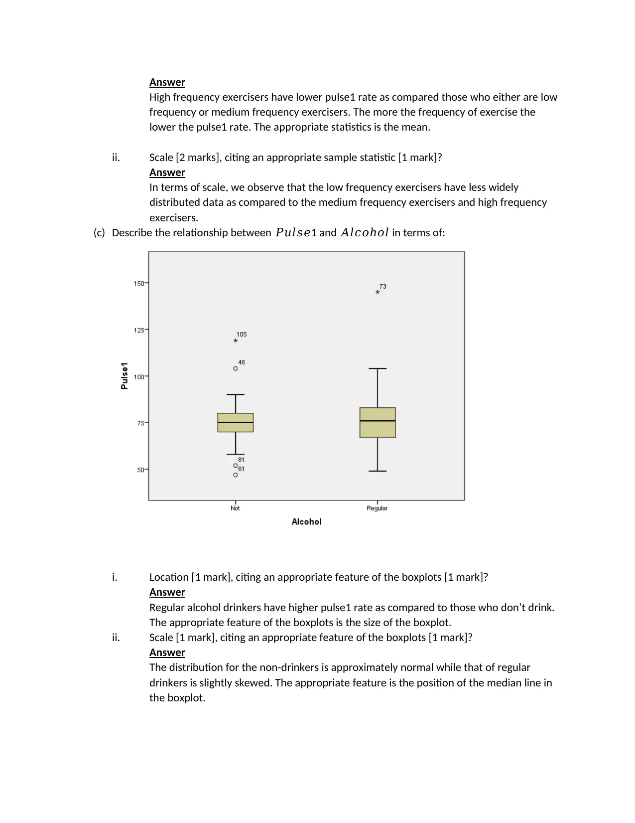
Descriptive Statistics: Pulse1
Variable Exercise N N* Mean SE Mean StDev Minimum Q1
Pulse1 High Frequency 14 0 68.64 3.39 12.69 49.00 59.00
Low Frequency 37 0 78.35 1.88 11.46 52.00 70.50
Medium Frequency 58 0 75.69 1.85 14.09 47.00 67.50
Variable Exercise Median Q3 Maximum
Pulse1 High Frequency 68.50 76.50 96.00
Low Frequency 78.00 85.00 119.00
Medium Frequency 75.00 80.50 145.00
i. Location [2 marks], citing an appropriate sample statistic [1 mark]?

Answer
High frequency exercisers have lower pulse1 rate as compared those who either are low
frequency or medium frequency exercisers. The more the frequency of exercise the
lower the pulse1 rate. The appropriate statistics is the mean.
ii. Scale [2 marks], citing an appropriate sample statistic [1 mark]?
Answer
In terms of scale, we observe that the low frequency exercisers have less widely
distributed data as compared to the medium frequency exercisers and high frequency
exercisers.
(c) Describe the relationship between 𝑃𝑢𝑙𝑠𝑒1 and 𝐴𝑙𝑐𝑜ℎ𝑜𝑙 in terms of:
i. Location [1 mark], citing an appropriate feature of the boxplots [1 mark]?
Answer
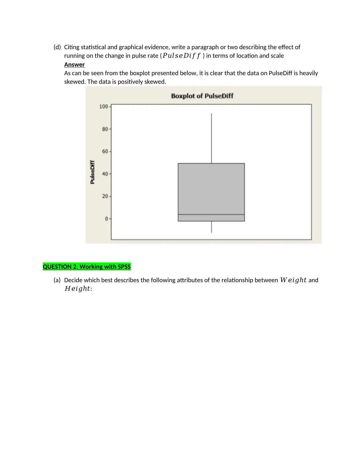
Regular alcohol drinkers have higher pulse1 rate as compared to those who don’t drink.
The appropriate feature of the boxplots is the size of the boxplot.
ii. Scale [1 mark], citing an appropriate feature of the boxplots [1 mark]?
Answer
The distribution for the non-drinkers is approximately normal while that of regular
drinkers is slightly skewed. The appropriate feature is the position of the median line in
the boxplot.

(d) Citing statistical and graphical evidence, write a paragraph or two describing the effect of
running on the change in pulse rate (𝑃𝑢𝑙𝑠𝑒𝐷𝑖𝑓𝑓 ) in terms of location and scale
Answer
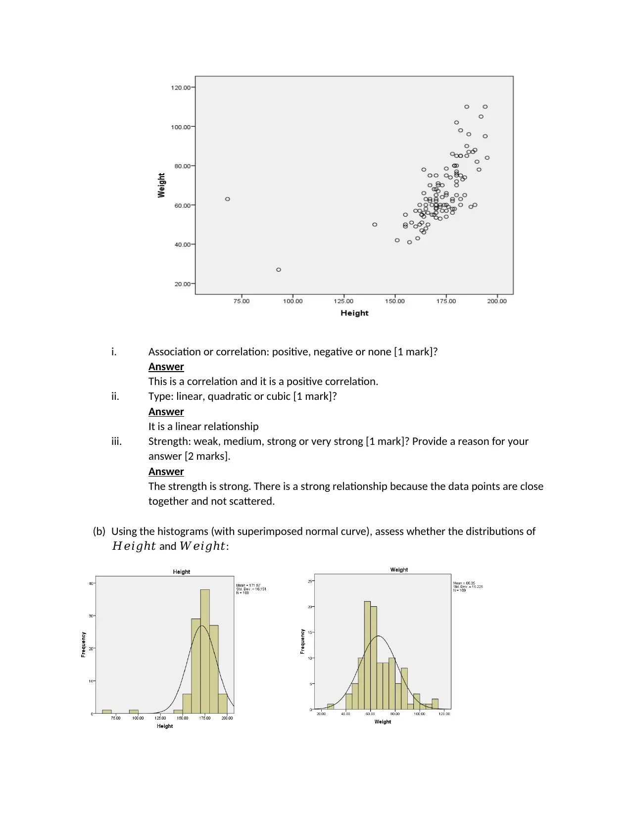
As can be seen from the boxplot presented below, it is clear that the data on PulseDiff is heavily
skewed. The data is positively skewed.
QUESTION 2. Working with SPSS
(a) Decide which best describes the following attributes of the relationship between 𝑊𝑒𝑖𝑔ℎ𝑡 and
𝐻𝑒𝑖𝑔ℎ𝑡:

i. Association or correlation: positive, negative or none [1 mark]?
Answer
This is a correlation and it is a positive correlation.
ii. Type: linear, quadratic or cubic [1 mark]?
Answer
It is a linear relationship
iii. Strength: weak, medium, strong or very strong [1 mark]? Provide a reason for your
answer [2 marks].
Answer
The strength is strong. There is a strong relationship because the data points are close
together and not scattered.
(b) Using the histograms (with superimposed normal curve), assess whether the distributions of
𝐻𝑒𝑖𝑔ℎ𝑡 and 𝑊𝑒𝑖𝑔ℎ𝑡:

i. Are located near the centre of the normal density curve [1 mark each]
Answer
The distribution of weight is located near the centre of the normal density curve while
that of height is located far away from the centre of the normal density curve.
ii. Are symmetrical like the normal density curve [1 mark each]
Answer
Weight has symmetrical like the normal density curve while height has asymmetrical
shape.
iii. Have too many outliers in comparison to the normal density curve [1 mark each]
Answer
Height has too many outliers in comparison to the normal density curve as compared to
the weight.
iv. And in conclusion look approximately normal [1 mark each].
Answer
In conclusion weight look to be approximately normal while height does not.
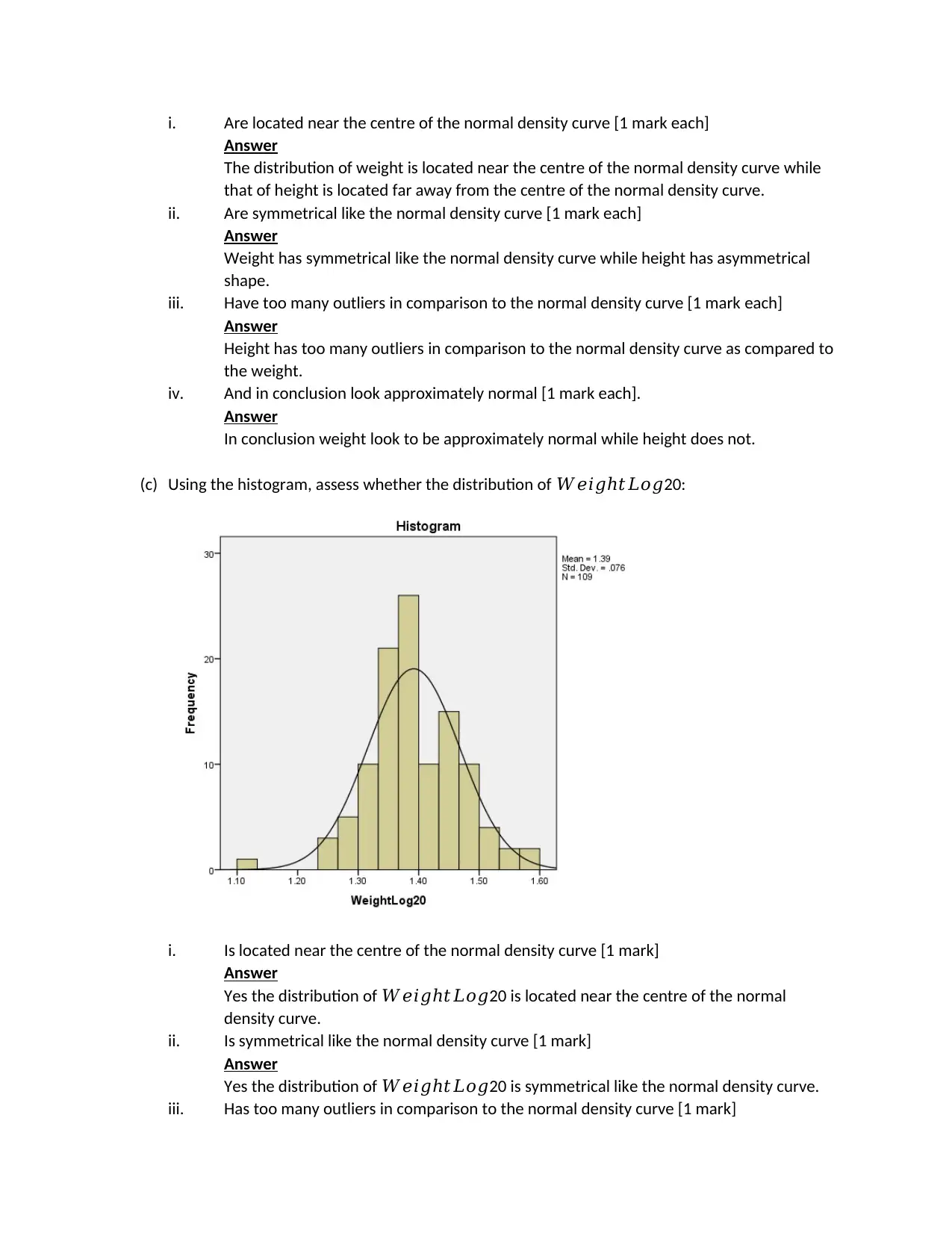
(c) Using the histogram, assess whether the distribution of 𝑊𝑒𝑖𝑔ℎ𝑡𝐿𝑜𝑔20:
i. Is located near the centre of the normal density curve [1 mark]
Answer
Yes the distribution of 𝑊𝑒𝑖𝑔ℎ𝑡𝐿𝑜𝑔20 is located near the centre of the normal
density curve.
ii. Is symmetrical like the normal density curve [1 mark]
Answer
Yes the distribution of 𝑊𝑒𝑖𝑔ℎ𝑡𝐿𝑜𝑔20 is symmetrical like the normal density curve.
iii. Has too many outliers in comparison to the normal density curve [1 mark]

Answer
There are no too many outliers for this distribution.
iv. And in conclusion looks approximately normal [1 mark].
Answer
In conclusion the distribution of 𝑊𝑒𝑖𝑔ℎ𝑡𝐿𝑜𝑔20 seem to be approximately normal.
(d) Writing your answer to 3 decimal places, calculate the regression model’s predicted value of
𝑊𝑒𝑖𝑔ℎ𝑡𝐿𝑜𝑔20 when 𝐻𝑒𝑖𝑔ℎ𝑡 = 183
Answer
WeightLog 20=0.473+ 0.005× Height
WeightLog 20=0.473+ 0.005× 183
WeightLog 20=0.473+ 0.915
WeightLog 20=1.388
(e) Recall the formula
WeightLog 20= loge (Weight )
loge (20)
WeightLog 20=1.388
1.388= loge ( Weight )
loge (20)
loge ( Weight )=1.388∗loge (20)
loge ( Weight ) =4.158076
x=eloge(x)=exp ¿
x=exp ¿