Data Management for Business Success: Analysis and Findings Report

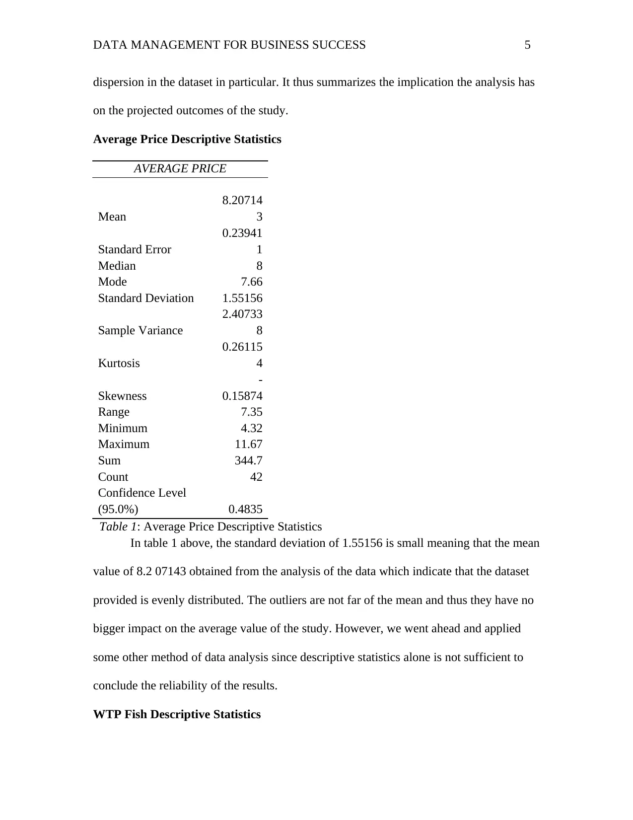
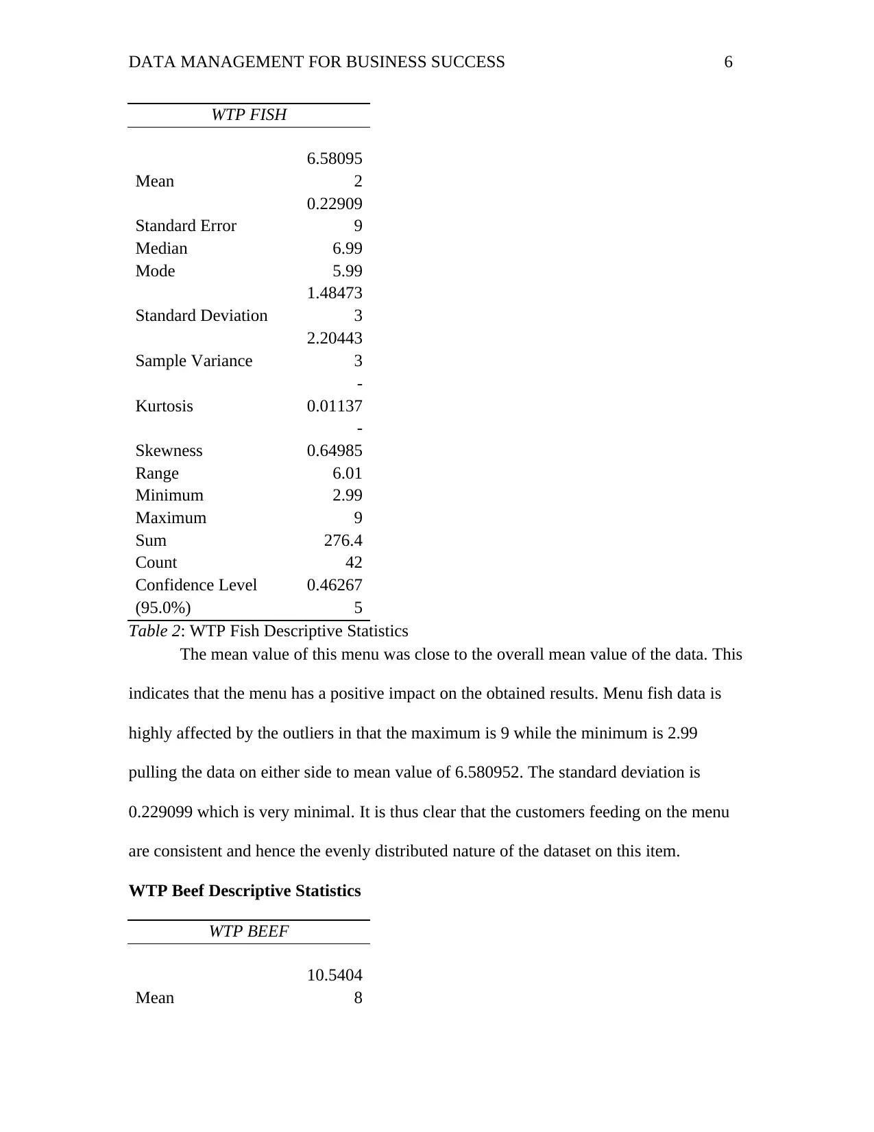
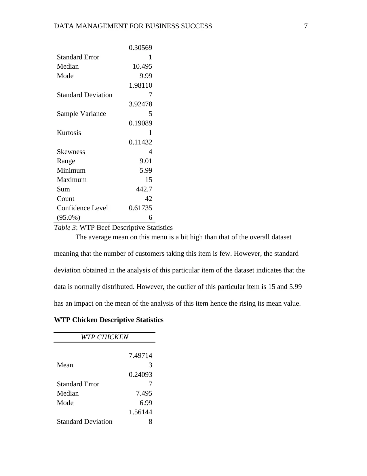
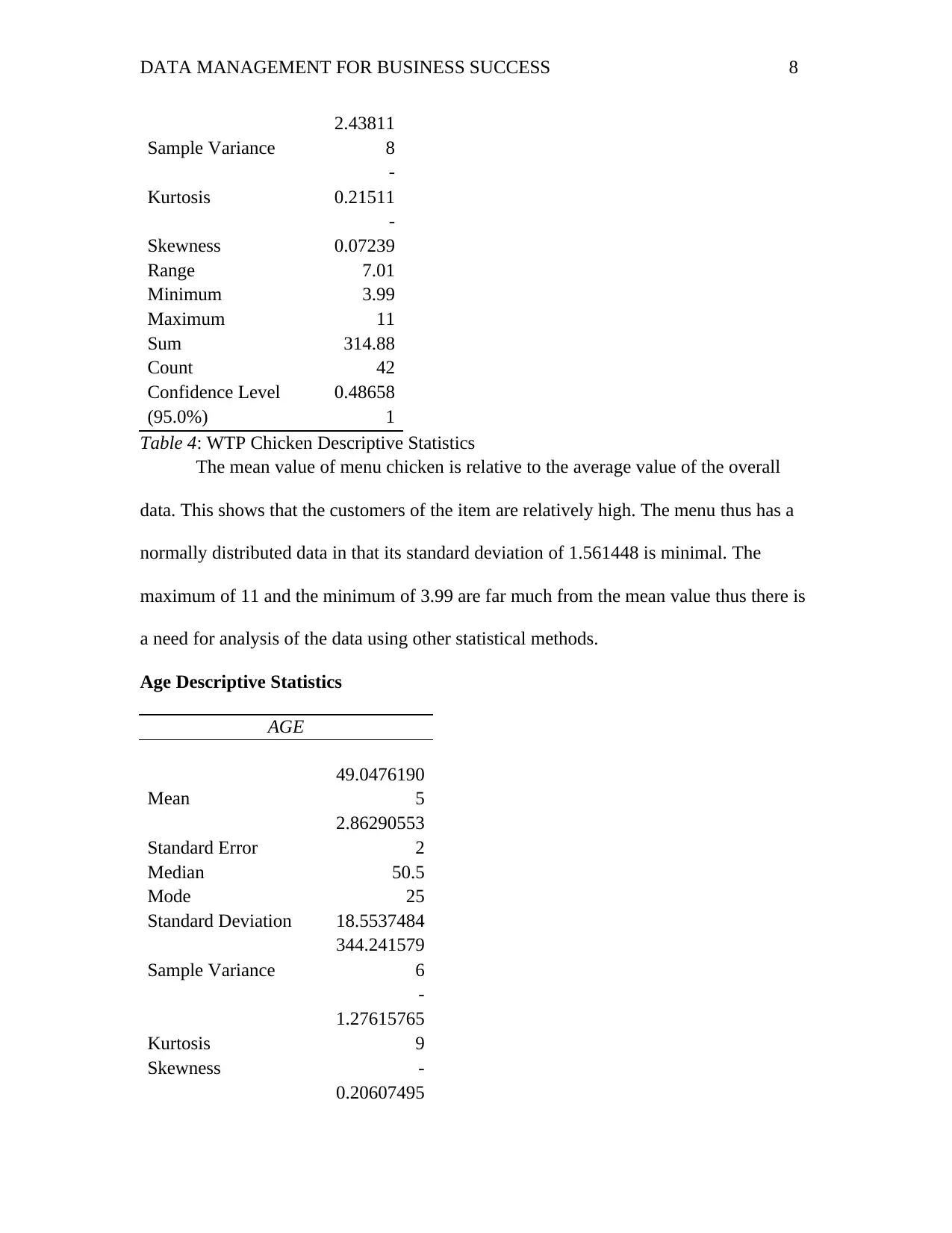
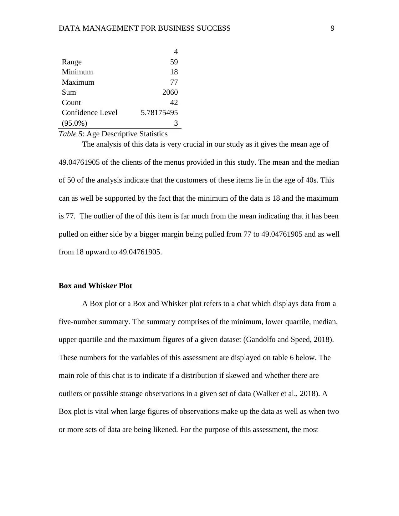
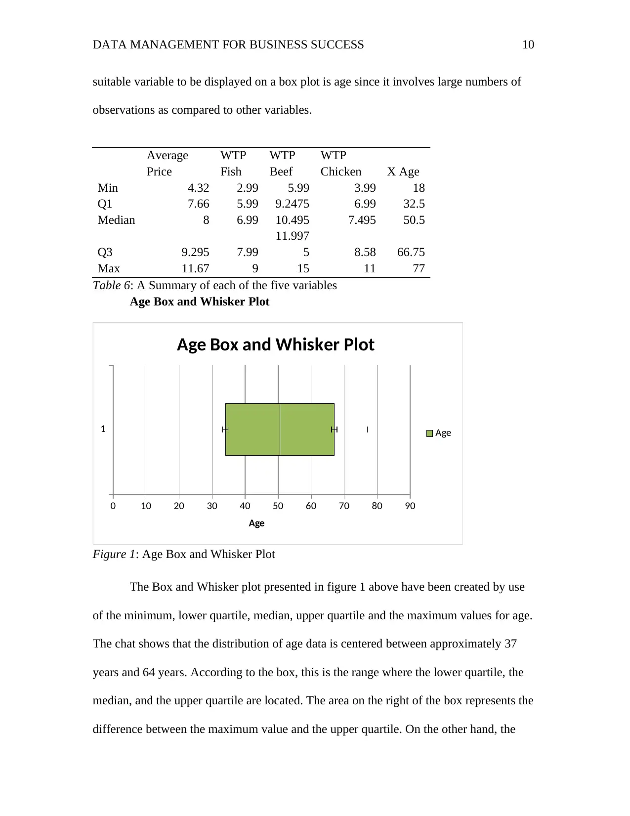
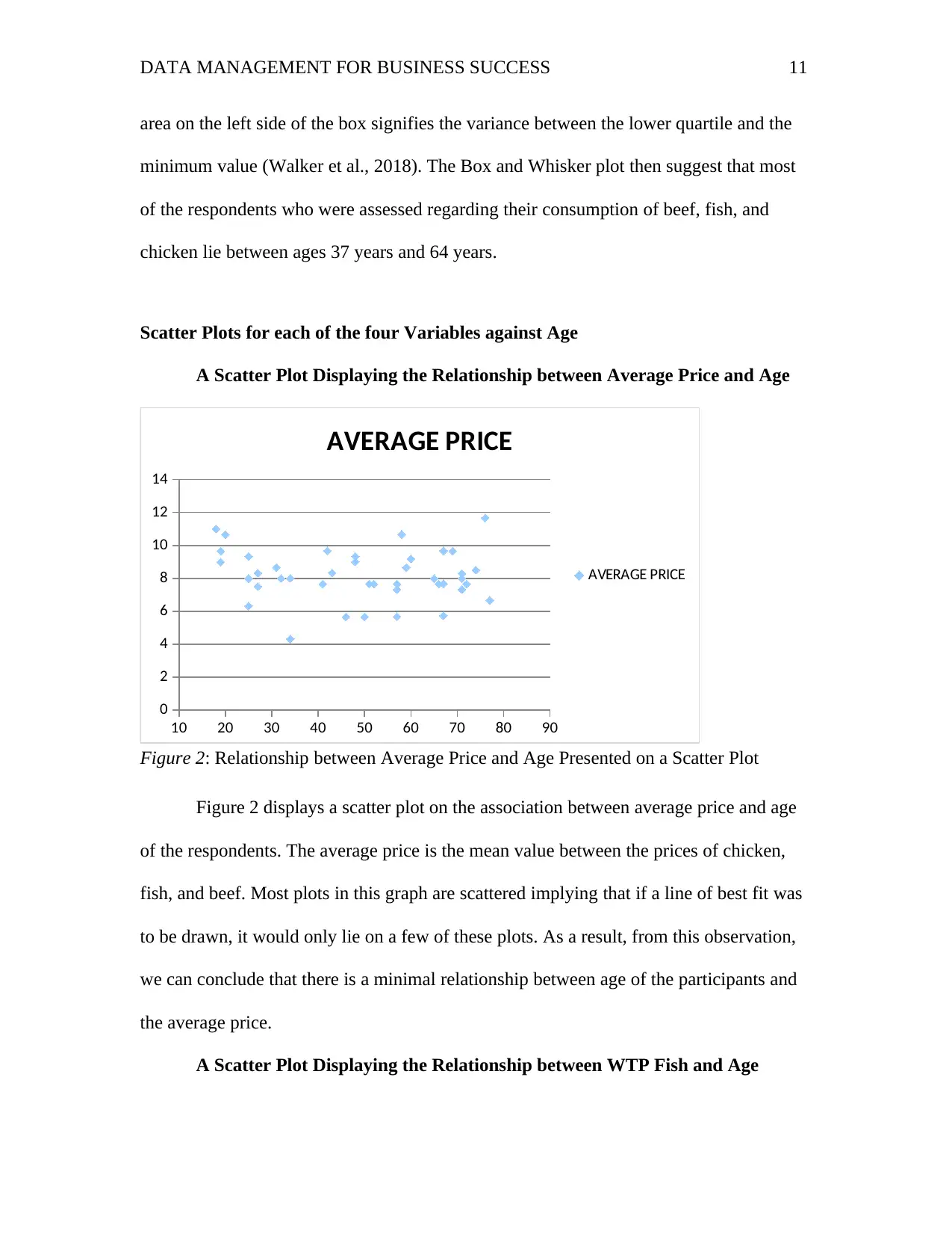
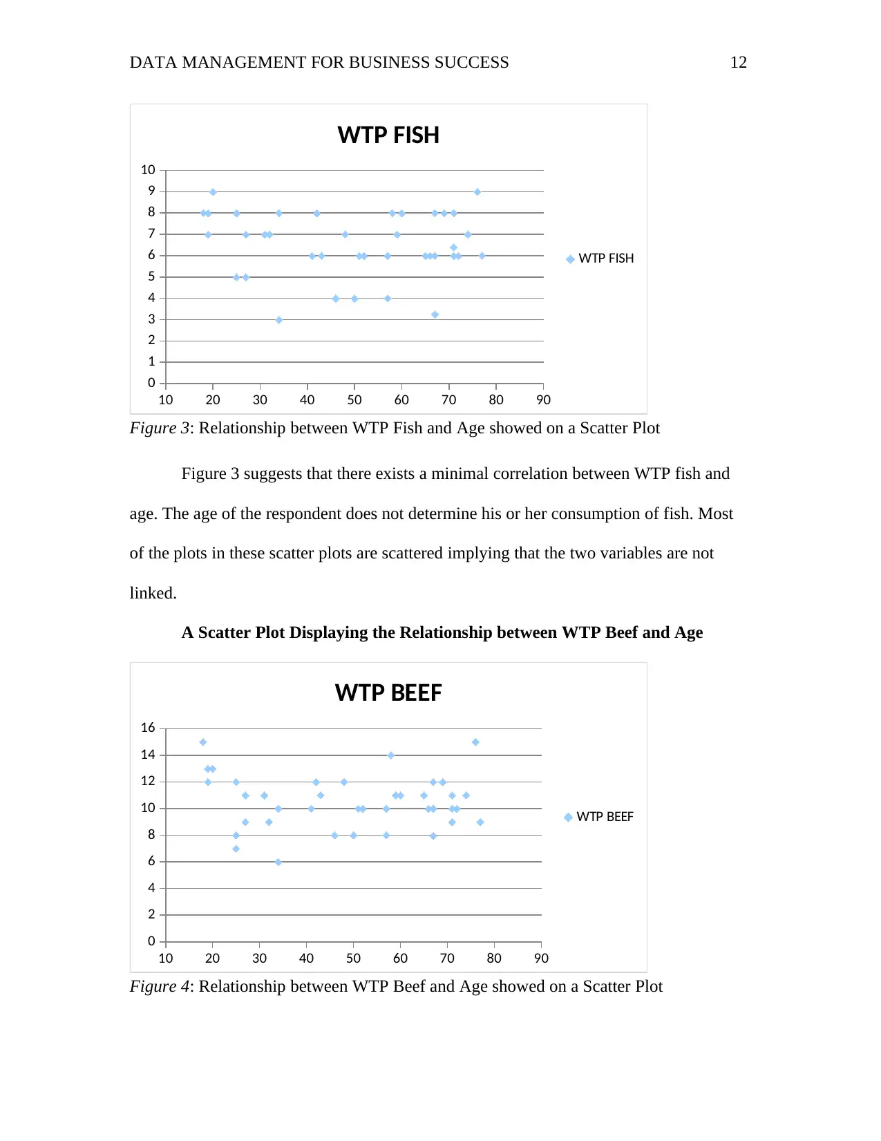
This report analyzes data management strategies for business success, focusing on a dataset related to restaurant menus and customer preferences. The analysis begins with data cleaning using Excel, addressing issues such as extra spacing, blank cells, and duplicate values. Descriptive statistics, including mean, standard deviation, median, mode, and range, are calculated for various parameters like average price, willingness to pay (WTP) for fish, beef, and chicken, and age. The report examines the distribution of the data and identifies potential outliers. Visual analysis is performed using box and whisker plots to illustrate the age distribution and scatter plots to explore the relationships between age and other variables like average price and WTP for each menu item. The findings indicate minimal correlations between age and the other variables. The report uses statistical methods and visual representations to provide a comprehensive overview of the data and its implications for business decision-making, highlighting the importance of data-driven insights for success in the hospitality industry.

Running head: DATA MANAGEMENT FOR BUSINESS SUCCESS 1
Data Management for Business Success
Student:
Professor:
Institution Affiliation:
Course:
Date:

DATA MANAGEMENT FOR BUSINESS SUCCESS 2
Table of Content
Table of Content..............................................................................................................................2
Introduction......................................................................................................................................3
Task I 4
Data Cleaning..................................................................................................................................4
Descriptive Statistics.......................................................................................................................4
Box and Whisker Plot......................................................................................................................8
Scatter Plots for each of the four Variables against Age...............................................................10
Age Pivot Table.............................................................................................................................13
A Histogram for Age.....................................................................................................................14

DATA MANAGEMENT FOR BUSINESS SUCCESS 3
Introduction
Online ordering of food has emerged a new platform for the big motels as well as
restaurants. Several people have welcomed the new innovation in the hospitality field
thus adopting the e-hotels. Further, the hotel owners have devised customer loyalty
through provision of coupons which have attracted even a bigger number in this e-
business service-delivery. The discovery has come in with advantages as it has created
opportunities for third-party companies. This has recorded the most prevailing and
rapidly growing business in the 21st century (Dalal & Sharma, 2018). Therefore, the
restaurant industries are recently known to popularly use internet tool for their business
activities. In this paper, we will discuss and analyze various popular menus frequency of
consumption and their average prices in some of the decent known restaurants in the
global market among people of various ages.
The data that was used in this analysis was obtained from various major hotels
and a sample population of 43 hotels and an equal number of people of different ages
against 3 popular menus (fish, chicken, and beef) was used in the study. The obtained
data were assessed and analyzed in the application of statistical tools. The analysis was
comprised of major statistical metrics such as descriptive statistics which evaluate for
mean, outliers, median, minimum as well as maximum values and also the standard
deviation and mode together with frequency distributions. Moreover, the visual analysis
of data involved correlation as well as inferential statistical methods.

DATA MANAGEMENT FOR BUSINESS SUCCESS 4
Task I
Data Cleaning
In statistics, data cleaning refers to a procedure or step by step method of getting
rid of invalid data present in a given dataset (Abedjan et al, 2016). There are several
processes that are involved depending on the hypothesis, as well as assumptions on
nature of the collected data. Usually, these data points are avoided and analysis is done
on the retained information. In the case of our provided study data, we will use the excel
data cleaning method in order to obtain a well organized and reliable dataset for analysis.
To achieve our objective of retrieving a usable dataset, a series of steps were
followed, which included: removing extra spacing in the data, selecting and treating all
cells that were blank, converting numeral values stored as text back into numbers,
removing all duplicate values, highlighting errors, changing the text to either lower or
upper or the proper case, parsing data by use of text to the column, spell checking,
deleting all formatting, and finally using find as well as replace (Chang & Myers, 2016).
The follow up of all these steps helped us to obtain the original data for analysis in our
study. These steps are only applicable in excel for the purposes of cleaning data for
statistical use.
Descriptive Statistics
The descriptive analysis involves or shows the following values of data analysis;
mean, standard deviation, range, median, range, mode, minimum, frequency distribution
as well as the maximum value of the data in a given study (Bhattacharyya, Bhattacharyya
& Kaur, 2018). This is simple displays the sense of values of central tendency and

DATA MANAGEMENT FOR BUSINESS SUCCESS 5
dispersion in the dataset in particular. It thus summarizes the implication the analysis has
on the projected outcomes of the study.
Average Price Descriptive Statistics
AVERAGE PRICE
Mean
8.20714
3
Standard Error
0.23941
1
Median 8
Mode 7.66
Standard Deviation 1.55156
Sample Variance
2.40733
8
Kurtosis
0.26115
4
Skewness
-
0.15874
Range 7.35
Minimum 4.32
Maximum 11.67
Sum 344.7
Count 42
Confidence Level
(95.0%) 0.4835
Table 1: Average Price Descriptive Statistics
In table 1 above, the standard deviation of 1.55156 is small meaning that the mean
value of 8.2 07143 obtained from the analysis of the data which indicate that the dataset
provided is evenly distributed. The outliers are not far of the mean and thus they have no
bigger impact on the average value of the study. However, we went ahead and applied
some other method of data analysis since descriptive statistics alone is not sufficient to
conclude the reliability of the results.
WTP Fish Descriptive Statistics

DATA MANAGEMENT FOR BUSINESS SUCCESS 6
WTP FISH
Mean
6.58095
2
Standard Error
0.22909
9
Median 6.99
Mode 5.99
Standard Deviation
1.48473
3
Sample Variance
2.20443
3
Kurtosis
-
0.01137
Skewness
-
0.64985
Range 6.01
Minimum 2.99
Maximum 9
Sum 276.4
Count 42
Confidence Level
(95.0%)
0.46267
5
Table 2: WTP Fish Descriptive Statistics
The mean value of this menu was close to the overall mean value of the data. This
indicates that the menu has a positive impact on the obtained results. Menu fish data is
highly affected by the outliers in that the maximum is 9 while the minimum is 2.99
pulling the data on either side to mean value of 6.580952. The standard deviation is
0.229099 which is very minimal. It is thus clear that the customers feeding on the menu
are consistent and hence the evenly distributed nature of the dataset on this item.
WTP Beef Descriptive Statistics
WTP BEEF
Mean
10.5404
8

DATA MANAGEMENT FOR BUSINESS SUCCESS 7
Standard Error
0.30569
1
Median 10.495
Mode 9.99
Standard Deviation
1.98110
7
Sample Variance
3.92478
5
Kurtosis
0.19089
1
Skewness
0.11432
4
Range 9.01
Minimum 5.99
Maximum 15
Sum 442.7
Count 42
Confidence Level
(95.0%)
0.61735
6
Table 3: WTP Beef Descriptive Statistics
The average mean on this menu is a bit high than that of the overall dataset
meaning that the number of customers taking this item is few. However, the standard
deviation obtained in the analysis of this particular item of the dataset indicates that the
data is normally distributed. However, the outlier of this particular item is 15 and 5.99
has an impact on the mean of the analysis of this item hence the rising its mean value.
WTP Chicken Descriptive Statistics
WTP CHICKEN
Mean
7.49714
3
Standard Error
0.24093
7
Median 7.495
Mode 6.99
Standard Deviation
1.56144
8

DATA MANAGEMENT FOR BUSINESS SUCCESS 8
Sample Variance
2.43811
8
Kurtosis
-
0.21511
Skewness
-
0.07239
Range 7.01
Minimum 3.99
Maximum 11
Sum 314.88
Count 42
Confidence Level
(95.0%)
0.48658
1
Table 4: WTP Chicken Descriptive Statistics
The mean value of menu chicken is relative to the average value of the overall
data. This shows that the customers of the item are relatively high. The menu thus has a
normally distributed data in that its standard deviation of 1.561448 is minimal. The
maximum of 11 and the minimum of 3.99 are far much from the mean value thus there is
a need for analysis of the data using other statistical methods.
Age Descriptive Statistics
AGE
Mean
49.0476190
5
Standard Error
2.86290553
2
Median 50.5
Mode 25
Standard Deviation 18.5537484
Sample Variance
344.241579
6
Kurtosis
-
1.27615765
9
Skewness -
0.20607495

DATA MANAGEMENT FOR BUSINESS SUCCESS 9
4
Range 59
Minimum 18
Maximum 77
Sum 2060
Count 42
Confidence Level
(95.0%)
5.78175495
3
Table 5: Age Descriptive Statistics
The analysis of this data is very crucial in our study as it gives the mean age of
49.04761905 of the clients of the menus provided in this study. The mean and the median
of 50 of the analysis indicate that the customers of these items lie in the age of 40s. This
can as well be supported by the fact that the minimum of the data is 18 and the maximum
is 77. The outlier of the of this item is far much from the mean indicating that it has been
pulled on either side by a bigger margin being pulled from 77 to 49.04761905 and as well
from 18 upward to 49.04761905.
Box and Whisker Plot
A Box plot or a Box and Whisker plot refers to a chat which displays data from a
five-number summary. The summary comprises of the minimum, lower quartile, median,
upper quartile and the maximum figures of a given dataset (Gandolfo and Speed, 2018).
These numbers for the variables of this assessment are displayed on table 6 below. The
main role of this chat is to indicate if a distribution if skewed and whether there are
outliers or possible strange observations in a given set of data (Walker et al., 2018). A
Box plot is vital when large figures of observations make up the data as well as when two
or more sets of data are being likened. For the purpose of this assessment, the most

DATA MANAGEMENT FOR BUSINESS SUCCESS 10
suitable variable to be displayed on a box plot is age since it involves large numbers of
observations as compared to other variables.
Average
Price
WTP
Fish
WTP
Beef
WTP
Chicken X Age
Min 4.32 2.99 5.99 3.99 18
Q1 7.66 5.99 9.2475 6.99 32.5
Median 8 6.99 10.495 7.495 50.5
Q3 9.295 7.99
11.997
5 8.58 66.75
Max 11.67 9 15 11 77
Table 6: A Summary of each of the five variables
Age Box and Whisker Plot
1
0 10 20 30 40 50 60 70 80 90
Age Box and Whisker Plot
Age
Age
Figure 1: Age Box and Whisker Plot
The Box and Whisker plot presented in figure 1 above have been created by use
of the minimum, lower quartile, median, upper quartile and the maximum values for age.
The chat shows that the distribution of age data is centered between approximately 37
years and 64 years. According to the box, this is the range where the lower quartile, the
median, and the upper quartile are located. The area on the right of the box represents the
difference between the maximum value and the upper quartile. On the other hand, the

DATA MANAGEMENT FOR BUSINESS SUCCESS 11
area on the left side of the box signifies the variance between the lower quartile and the
minimum value (Walker et al., 2018). The Box and Whisker plot then suggest that most
of the respondents who were assessed regarding their consumption of beef, fish, and
chicken lie between ages 37 years and 64 years.
Scatter Plots for each of the four Variables against Age
A Scatter Plot Displaying the Relationship between Average Price and Age
10 20 30 40 50 60 70 80 90
0
2
4
6
8
10
12
14
AVERAGE PRICE
AVERAGE PRICE
Figure 2: Relationship between Average Price and Age Presented on a Scatter Plot
Figure 2 displays a scatter plot on the association between average price and age
of the respondents. The average price is the mean value between the prices of chicken,
fish, and beef. Most plots in this graph are scattered implying that if a line of best fit was
to be drawn, it would only lie on a few of these plots. As a result, from this observation,
we can conclude that there is a minimal relationship between age of the participants and
the average price.
A Scatter Plot Displaying the Relationship between WTP Fish and Age

DATA MANAGEMENT FOR BUSINESS SUCCESS 12
10 20 30 40 50 60 70 80 90
0
1
2
3
4
5
6
7
8
9
10
WTP FISH
WTP FISH
Figure 3: Relationship between WTP Fish and Age showed on a Scatter Plot
Figure 3 suggests that there exists a minimal correlation between WTP fish and
age. The age of the respondent does not determine his or her consumption of fish. Most
of the plots in these scatter plots are scattered implying that the two variables are not
linked.
A Scatter Plot Displaying the Relationship between WTP Beef and Age
10 20 30 40 50 60 70 80 90
0
2
4
6
8
10
12
14
16
WTP BEEF
WTP BEEF
Figure 4: Relationship between WTP Beef and Age showed on a Scatter Plot