Simple Linear Regression Model and Data Analysis Report

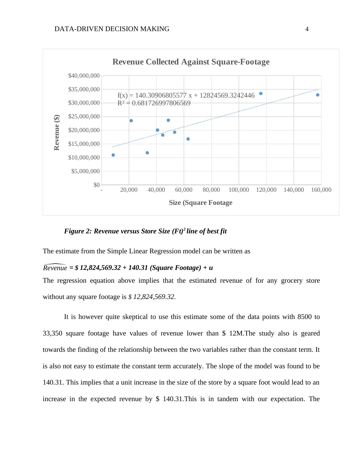
This report presents a data-driven analysis of the relationship between a grocery store's square footage and its revenue. Using a dataset of ten locations, a simple linear regression model was employed to determine the correlation between these two variables. The analysis involved creating scatter plots, deriving a regression equation (Revenue = $12,824,569.32 + 140.31(Square Footage)), and calculating an R-squared value of 0.68. This indicates that 68% of the variation in revenue can be attributed to changes in store size. The report discusses the implications of the positive relationship between store size and revenue, as well as the influence of other factors affecting revenue, such as distance, security, and social amenities. The report also addresses the model's limitations and provides insights into the practical application of the findings for decision-making.

Running Head: DATA-DRIVEN DECISION MAKING 1
Data-Driven Decision Making
Student’s Name
Institutional Affiliation

DATA-DRIVEN DECISION MAKING 2
Data-Driven Decision Making
According to Mulholland & Jones (2013) for a simple regression model, the equation is
written as; Y= b0+ b1 X1 + u Where Y-is the Predicted variable, b0 and b1–are constants, u =
Random Error and X1- is the predictor variable.
In this analysis, we are interested in finding out the relationship that exists between Revenue
collected from individual Big Grocery stores by location and Big Grocery store square footage
by location. In this case, it is assumed that the revenue collected from the grocery store depends
on the square footage of the store. Therefore, revenue is the dependent variable while size
(square footage) is the independent variable. Here, we will try to unravel if the revenue collected
is influenced by the size of the grocery store. Below is the sample data for analysis.
Table 1: Sample Data
Location Square Footage (x) Revenue (y)
Location 1 48,720.39 $23,665,319.22
Location 2 40,778.72 $20,066,838.98
Location 3 21,654.19 $23,508,691.46
Location 4 33,344.11 $11,748,300.32
Location 5 116,006.40 $33,450,105.86
Location 6 44,655.98 $18,248,754.69
Location 7 8,549.08 $10,943,196.86
Location 8 157,424.48 $32,934,788.04
Location 9 63,075.32 $16,821,187.57
Location 10 53,256.79 $19,285,241.45
From the dataset above, a scatter plot was drawn using excel to show how the data points
were distributed in the chart. This shows a visual display of the direction and likely strength of
the relationship between the two variable. According to figure 1, the data points are clustered
from the left side to the right side, which shows a positive slope (positive relationship).

DATA-DRIVEN DECISION MAKING 3
- 20,000 40,000 60,000 80,000 100,000 120,000 140,000 160,000
$0
$5,000,000
$10,000,000
$15,000,000
$20,000,000
$25,000,000
$30,000,000
$35,000,000
$40,000,000
Revenue Collected Against Square-Footage
Size (Square Footage)
Revenue ($)
Figure 1: Revenue versus Store Size (Ft)2 Scatter plot
The figure 2 below shows the scatter plot above data fitted with the line of best fit. This is
commonly referred to as the trend line. The trend line affirms the existence of a positive
relationship between the two variables. The regression equation for this experiment can be
written as;
Revenue= b0+ b1 (Square Footage) + u

DATA-DRIVEN DECISION MAKING 4
- 20,000 40,000 60,000 80,000 100,000 120,000 140,000 160,000
$0
$5,000,000
$10,000,000
$15,000,000
$20,000,000
$25,000,000
$30,000,000
$35,000,000
$40,000,000
f(x) = 140.30906805577 x + 12824569.3242446
R² = 0.681726997806569
Revenue Collected Against Square-Footage
Size (Square Footage
Revenue ($)
Figure 2: Revenue versus Store Size (Ft)2 line of best fit
The estimate from the Simple Linear Regression model can be written as
^Revenue = $ 12,824,569.32 + 140.31 (Square Footage) + u
The regression equation above implies that the estimated revenue of for any grocery store
without any square footage is $ 12,824,569.32.
It is however quite skeptical to use this estimate some of the data points with 8500 to
33,350 square footage have values of revenue lower than $ 12M.The study also is geared
towards the finding of the relationship between the two variables rather than the constant term. It
is also not easy to estimate the constant term accurately. The slope of the model was found to be
140.31. This implies that a unit increase in the size of the store by a square foot would lead to an
increase in the expected revenue by $ 140.31.This is in tandem with our expectation. The

DATA-DRIVEN DECISION MAKING 5
positive relationship shows that the revenue amounts increases as the size of the store (square
footage) increases and vice versa.
The R-Squared value of the model was found to be 0.68. This implies that 68% of the variation
in grocery stores revenue can be attributed to the changes in the stores' footage (Berenson, et al,
2012). The remaining 32% of the variation is attributed to errors and other factors outside the
model that affect revenue such as distance, securities and other social amenities available in the
area.
In summary, we can categorize the findings into;
 Linear in Parameters
In regression analysis, the regression line rarely passes through each point in the data plotted
until there is a perfect correlation (Cox, 2018). Considering that the y values are normally
predicted, and the data that is normally used is actual observed items, it results in a difference
that arises between the values of y that are predicted and observed. The differences between the
two are known as residuals (observed y - expected y). The points lying above the line of best fit
will result in positive residuals while they that lie below are negative residuals. In figure 2, both
positive and negative residuals are observed. According to the scatter plot in figure 1, there is a
strong correlation between the revenue and the size and square footage by location. The
distances to the line of best fit are minimal. The assumption of linearity is met from the analysis
above since the data points are clustered along the line of best fit (Larson, & Farber, 2019).
 Random Sampling
This is a method of probability sampling where each item in the population has equal chances of
being selected in the sample. From an overview of the data set provided, randomness was

DATA-DRIVEN DECISION MAKING 6
observed when selecting the sample data to be used. A clear positive relationship can be
observed easily even prior analysis since the high revenue was realized in areas with huge square
footage. The data set comprised of 10 locations that seem to have been selected randomly in a
city since there seems to be a fluctuation. If this were not the case, a similar pattern would be
observed in the data set from location 1 to location 10.
 Sample Variation in the Explanatory Variable
Considering the sample size of 10, which is relatively small, instances in data variation can
be observed. As the sample size increases, the sample approaches the population hence data
variation reduces. There is a lot of missing data between 60,000 to 120,000 square foot there
could have influenced the direction of the relationship. Nonetheless, a line of best fit can be fitted
with at least 3 points hence the data is still sufficient estimator of the impact of store square foot
on revenue.
 Zero mean of the error term conditional on the independent variable
The error term (u) suggest that there exist numerous variables that affect grocery stores
revenue apart from the square foot. The R-Squared value of the model was found to be 0.68,
which shows that only 68% of the variation in grocery stores revenue can be attributed to the
changes in the stores' footage. The remaining 32% of the variation is attributed to errors and
other factors outside the model that affect revenue such as distance, security among others
(Sullivan & Verhoosel,2013). This being the case, one would not take the estimate of revenue
too strictly. However,68% estimate is statistically viable (Gupta and Kapoor, 2019).

DATA-DRIVEN DECISION MAKING 7
In conclusion, the model is a sufficient estimator of revenue. A high correlation between
revenue and square foot was realized. The two variables were also positively related.
References
Berenson, M., Levine, D., Szabat, K. A., & Krehbiel, T. C. (2012). Basic business statistics:
Concepts and applications. Pearson higher education AU.
Cox, D. R. (2018). Applied statistics-principles and examples. Routledge.
Groebner, D. F., Shannon, P. W., Fry, P. C., & Smith, K. D. (2013). Business statistics. Pearson
Education UK.
Gupta, S.C. and Kapoor, V.K. (2019), Fundamentals of applied statistics. Sulthan Chand &
Sons.
Larson, R., & Farber, B. (2019). Elementary statistics. Pearson.
McClave, J. T., Benson, P. G., Sincich, T., & Sincich, T. (2014). Statistics for business and
economics. Boston: Pearson.
Mulholland, H., & Jones, C. R. (2013). Fundamentals of statistics. Springer.
Napier, C., & Maisel, J. W.(2015), Principles and Procedures of Statistics: a Biometric
Approach. McGraw Hill Book Company, New York.
Sullivan, M., & Verhoosel, J. C. M. (2013). Statistics: Informed decisions using data. New York:
Pearson.

DATA-DRIVEN DECISION MAKING 8