Data Exploration and Preparation Report: Analysis of Marketing Data

This report presents a comprehensive analysis of data exploration and preparation techniques applied to a marketing dataset. It begins with an initial data exploration, identifying attribute types and calculating descriptive statistics, including counts, frequencies, and summary statistics for both categorical and numerical variables. The analysis then delves into data exploration using the KNIME analytics platform, which involves coding categorical attributes, identifying outliers, and performing cross-tabulation to reveal relationships between variables, such as marital status and education level, day of the week contacted and campaign outcome, and day of the week contacted and subscription status. Furthermore, Pearson correlation and regression estimation are applied to ratio attributes for further insights. Finally, the report covers data processing techniques, including binning, normalization, discretization, and binarization, to prepare the data for further analysis and modeling. The report aims to provide a detailed understanding of the data and the steps involved in preparing it for advanced analytics.

Data Exploration 1
DATA EXPLORATION AND PREPARATION
by[Name]
Course
Professor’s Name
Institution
Location of Institution
Date

Data Exploration 2
Contents of Contents
Contents of Contents..................................................................................................................2
A1. Initial Data exploration........................................................................................................3
1. Type of Attributes............................................................................................................3
2. Descriptive Statistics.......................................................................................................3
Percentage and Counts for Categorical Data....................................................................3
Summary Statistics for Interval and Ratio Variables.........................................................7
3. Exploration of Data.........................................................................................................8
Coding Categorical Attributes............................................................................................8
Outliers...............................................................................................................................9
Cross - Tabulation............................................................................................................10
Pearson correlation on Ratio Attributes...........................................................................14
Regression Estimation......................................................................................................14
1B. Data Processing.................................................................................................................17
(a) Binning......................................................................................................................17
(b) Normalisation............................................................................................................17
(c) Discretise...................................................................................................................18
(d) Binarise......................................................................................................................18
1C. Summary............................................................................................................................19

Data Exploration 3
Data Exploration and Preparation
A1. Initial Data exploration
1. Type of Attributes
Type of job, Marital status, Default, Housing, Loan, contact, poutcome are nominal
measurement scale, in which numbers serve as “tags” or “labels” only, to identify or classify
the objects. A nominal scale measurement normally deals with measurements in which
numbers have no value. Education, month, and day of week are ordinal measurement scale
since variables reports the ranking and ordering of the data without actually establishing the
degree of variation between them. Duration, campaign, pdays, and previous are interval
measurement scale since the difference between two variables is meaningful. Finally, age,
Empty.var.rate, cons.price.idx, cons.conf.idx, euribor3m, nr.employed, and y are ratio
measurement scale since the zero point make sense.
2. Descriptive Statistics
Descriptive statistics include measures of central tendency, dispersions and frequencies.
For interval and ratio variables measures of central tendency and dispersion are used to
summarize the data. However, for nominal and ordinal variables counts and frequencies are
used. The nominal and ordinal data re coded as follows:
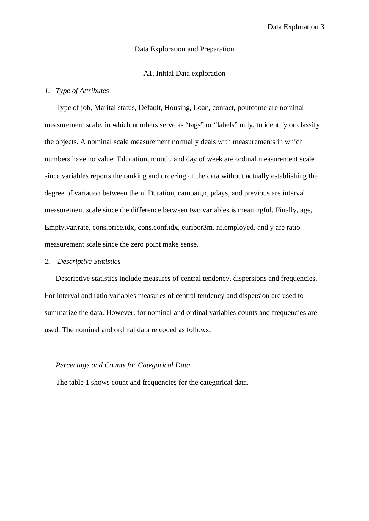
Percentage and Counts for Categorical Data
The table 1 shows count and frequencies for the categorical data.

Data Exploration 4
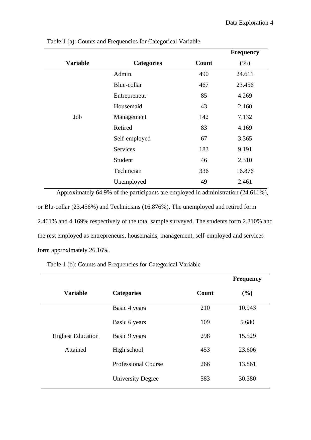
Table 1 (a): Counts and Frequencies for Categorical Variable
Variable Categories Count
Frequency
(%)
Admin. 490 24.611
Blue-collar 467 23.456
Entrepreneur 85 4.269
Housemaid 43 2.160
Job Management 142 7.132
Retired 83 4.169
Self-employed 67 3.365
Services 183 9.191
Student 46 2.310
Technician 336 16.876
Unemployed 49 2.461
Approximately 64.9% of the participants are employed in administration (24.611%),
or Blu-collar (23.456%) and Technicians (16.876%). The unemployed and retired form
2.461% and 4.169% respectively of the total sample surveyed. The students form 2.310% and
the rest employed as entrepreneurs, housemaids, management, self-employed and services
form approximately 26.16%.
Table 1 (b): Counts and Frequencies for Categorical Variable
Variable Categories Count
Frequency
(%)
Basic 4 years 210 10.943
Basic 6 years 109 5.680
Highest Education Basic 9 years 298 15.529
Attained High school 453 23.606
Professional Course 266 13.861
University Degree 583 30.380

Data Exploration 5
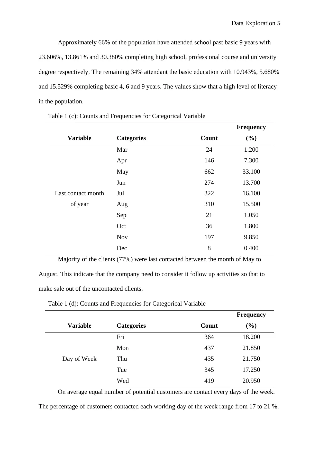
Approximately 66% of the population have attended school past basic 9 years with
23.606%, 13.861% and 30.380% completing high school, professional course and university
degree respectively. The remaining 34% attendant the basic education with 10.943%, 5.680%
and 15.529% completing basic 4, 6 and 9 years. The values show that a high level of literacy
in the population.
Table 1 (c): Counts and Frequencies for Categorical Variable
Variable Categories Count
Frequency
(%)
Mar 24 1.200
Apr 146 7.300
May 662 33.100
Jun 274 13.700
Last contact month Jul 322 16.100
of year Aug 310 15.500
Sep 21 1.050
Oct 36 1.800
Nov 197 9.850
Dec 8 0.400
Majority of the clients (77%) were last contacted between the month of May to
August. This indicate that the company need to consider it follow up activities so that to
make sale out of the uncontacted clients.
Table 1 (d): Counts and Frequencies for Categorical Variable
Variable Categories Count
Frequency
(%)
Fri 364 18.200
Mon 437 21.850
Day of Week Thu 435 21.750
Tue 345 17.250
Wed 419 20.950
On average equal number of potential customers are contact every days of the week.
The percentage of customers contacted each working day of the week range from 17 to 21 %.

Data Exploration 6
Table 1 (e): Counts and Frequencies for Categorical Variable
Variable Categories Count
Frequency
(%)
Divorced 229 11.461
Marital Status Married 1240 62.062
Single 529 26.476
Outcome of the
previous Failure 197 9.850
marketing campaign Non-existent 1741 87.050
Success 62 3.100
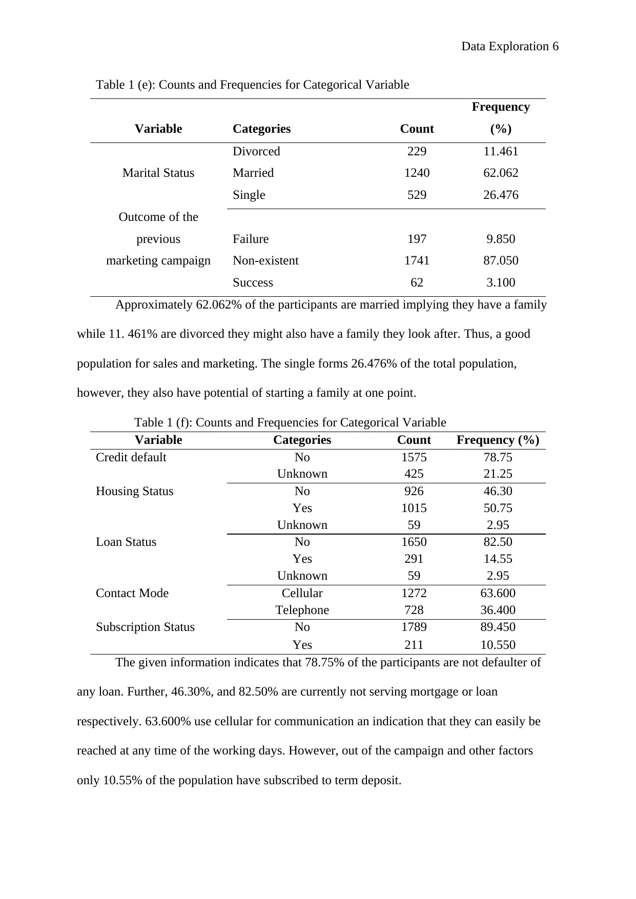
Approximately 62.062% of the participants are married implying they have a family
while 11. 461% are divorced they might also have a family they look after. Thus, a good
population for sales and marketing. The single forms 26.476% of the total population,
however, they also have potential of starting a family at one point.
Table 1 (f): Counts and Frequencies for Categorical Variable
Variable Categories Count Frequency (%)
Credit default No
Unknown
1575
425
78.75
21.25
Housing Status No 926 46.30
Yes
Unknown
1015
59
50.75
2.95
Loan Status No 1650 82.50
Yes
Unknown
291
59
14.55
2.95
Contact Mode Cellular 1272 63.600
Telephone [phone]
Subscription Status No 1789 89.450
Yes 211 10.550
The given information indicates that 78.75% of the participants are not defaulter of
any loan. Further, 46.30%, and 82.50% are currently not serving mortgage or loan
respectively. 63.600% use cellular for communication an indication that they can easily be
reached at any time of the working days. However, out of the campaign and other factors
only 10.55% of the population have subscribed to term deposit.

Data Exploration 7
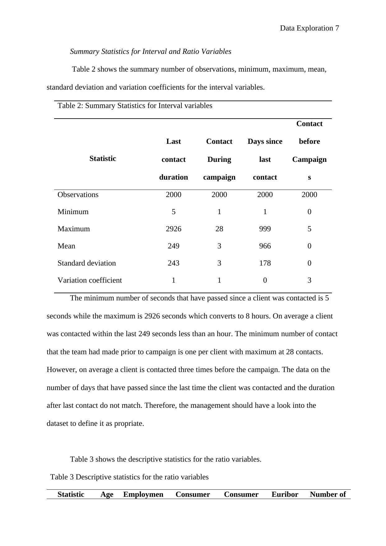
Summary Statistics for Interval and Ratio Variables
Table 2 shows the summary number of observations, minimum, maximum, mean,
standard deviation and variation coefficients for the interval variables.
Table 2: Summary Statistics for Interval variables
Statistic
Last
contact
duration
Contact
During
campaign
Days since
last
contact
Contact
before
Campaign
s
Observations 2000 2000 2000 2000
Minimum 5 1 1 0
Maximum 2926 28 999 5
Mean 249 3 966 0
Standard deviation 243 3 178 0
Variation coefficient 1 1 0 3
The minimum number of seconds that have passed since a client was contacted is 5
seconds while the maximum is 2926 seconds which converts to 8 hours. On average a client
was contacted within the last 249 seconds less than an hour. The minimum number of contact
that the team had made prior to campaign is one per client with maximum at 28 contacts.
However, on average a client is contacted three times before the campaign. The data on the
number of days that have passed since the last time the client was contacted and the duration
after last contact do not match. Therefore, the management should have a look into the
dataset to define it as propriate.
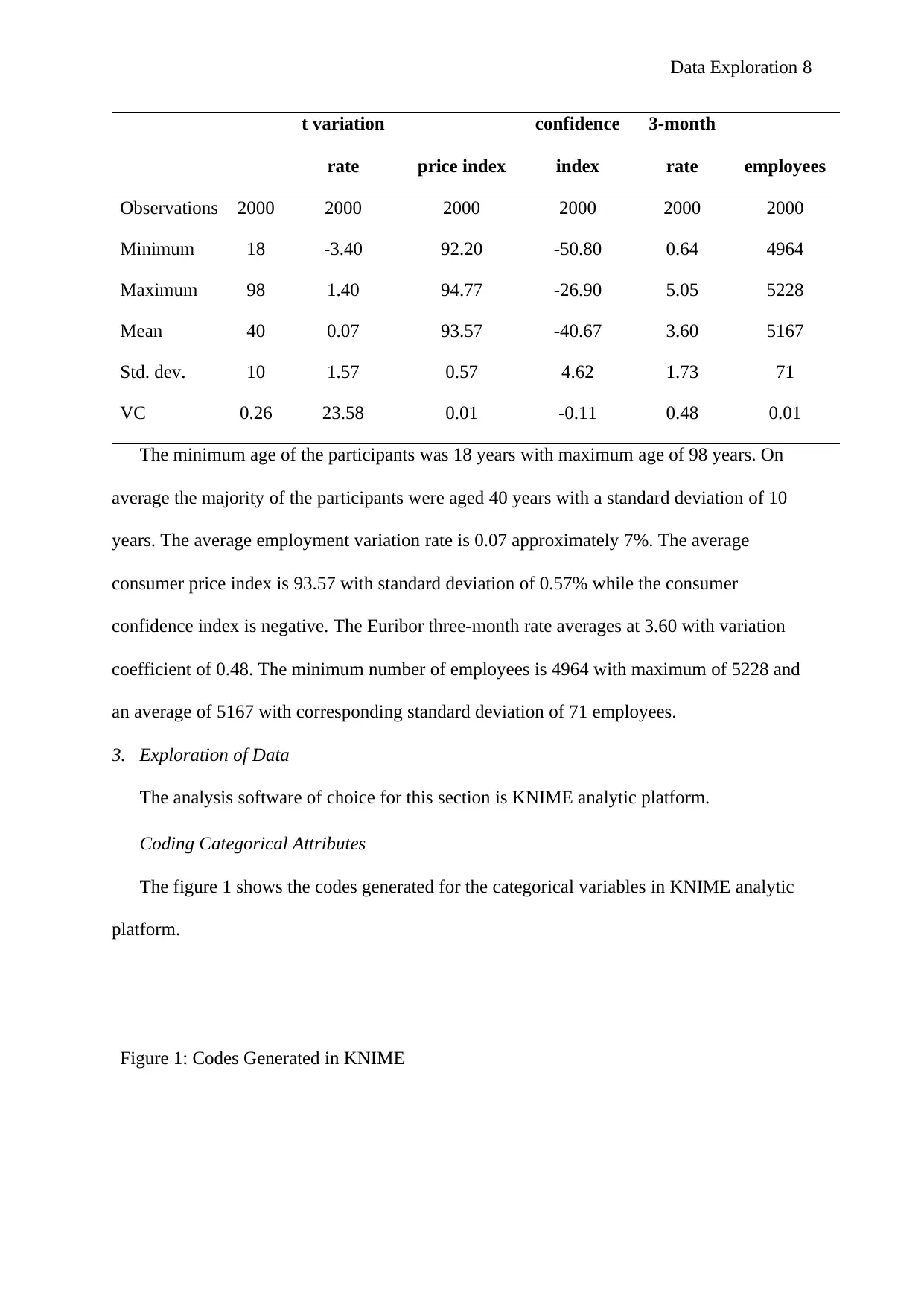
Table 3 shows the descriptive statistics for the ratio variables.
Table 3 Descriptive statistics for the ratio variables
Statistic Age Employmen Consumer Consumer Euribor Number of

Data Exploration 8
t variation
rate price index
confidence
index
3-month
rate employees
Observations 2000 2000 2000 2000 2000 2000
Minimum 18 -3.40 92.20 -50.80 0.64 4964
Maximum 98 1.40 94.77 -26.90 5.05 5228
Mean 40 0.07 93.57 -40.67 3.60 5167
Std. dev. 10 1.57 0.57 4.62 1.73 71
VC 0.26 23.58 0.01 -0.11 0.48 0.01
The minimum age of the participants was 18 years with maximum age of 98 years. On
average the majority of the participants were aged 40 years with a standard deviation of 10
years. The average employment variation rate is 0.07 approximately 7%. The average
consumer price index is 93.57 with standard deviation of 0.57% while the consumer
confidence index is negative. The Euribor three-month rate averages at 3.60 with variation
coefficient of 0.48. The minimum number of employees is 4964 with maximum of 5228 and
an average of 5167 with corresponding standard deviation of 71 employees.
3. Exploration of Data
The analysis software of choice for this section is KNIME analytic platform.
Coding Categorical Attributes
The figure 1 shows the codes generated for the categorical variables in KNIME analytic
platform.
Figure 1: Codes Generated in KNIME

Data Exploration 9
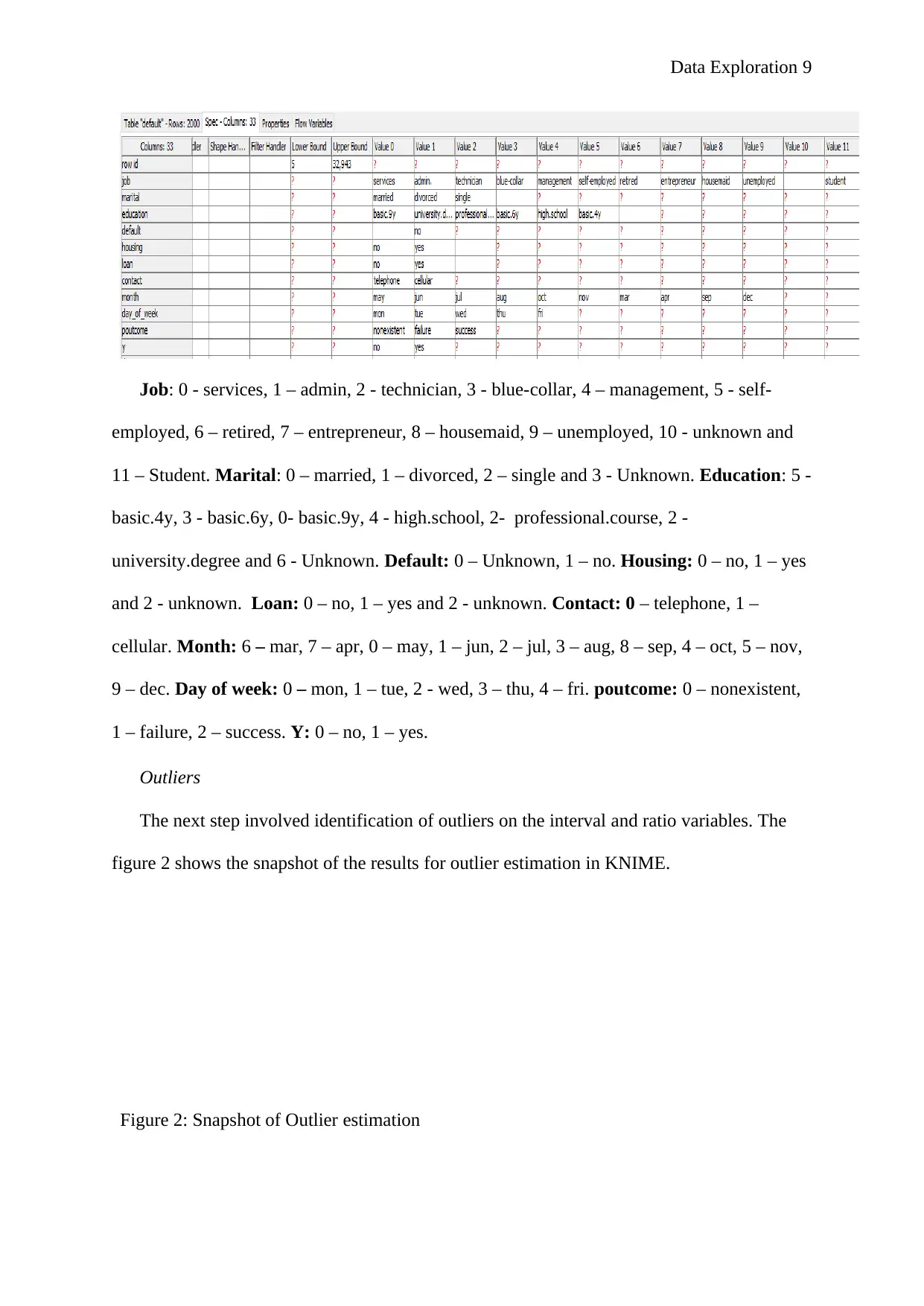
Job: 0 - services, 1 – admin, 2 - technician, 3 - blue-collar, 4 – management, 5 - self-
employed, 6 – retired, 7 – entrepreneur, 8 – housemaid, 9 – unemployed, 10 - unknown and
11 – Student. Marital: 0 – married, 1 – divorced, 2 – single and 3 - Unknown. Education: 5 -
basic.4y, 3 - basic.6y, 0- basic.9y, 4 - high.school, 2- professional.course, 2 -
university.degree and 6 - Unknown. Default: 0 – Unknown, 1 – no. Housing: 0 – no, 1 – yes
and 2 - unknown. Loan: 0 – no, 1 – yes and 2 - unknown. Contact: 0 – telephone, 1 –
cellular. Month: 6 – mar, 7 – apr, 0 – may, 1 – jun, 2 – jul, 3 – aug, 8 – sep, 4 – oct, 5 – nov,
9 – dec. Day of week: 0 – mon, 1 – tue, 2 - wed, 3 – thu, 4 – fri. poutcome: 0 – nonexistent,
1 – failure, 2 – success. Y: 0 – no, 1 – yes.
Outliers
The next step involved identification of outliers on the interval and ratio variables. The
figure 2 shows the snapshot of the results for outlier estimation in KNIME.
Figure 2: Snapshot of Outlier estimation

Data Exploration 10
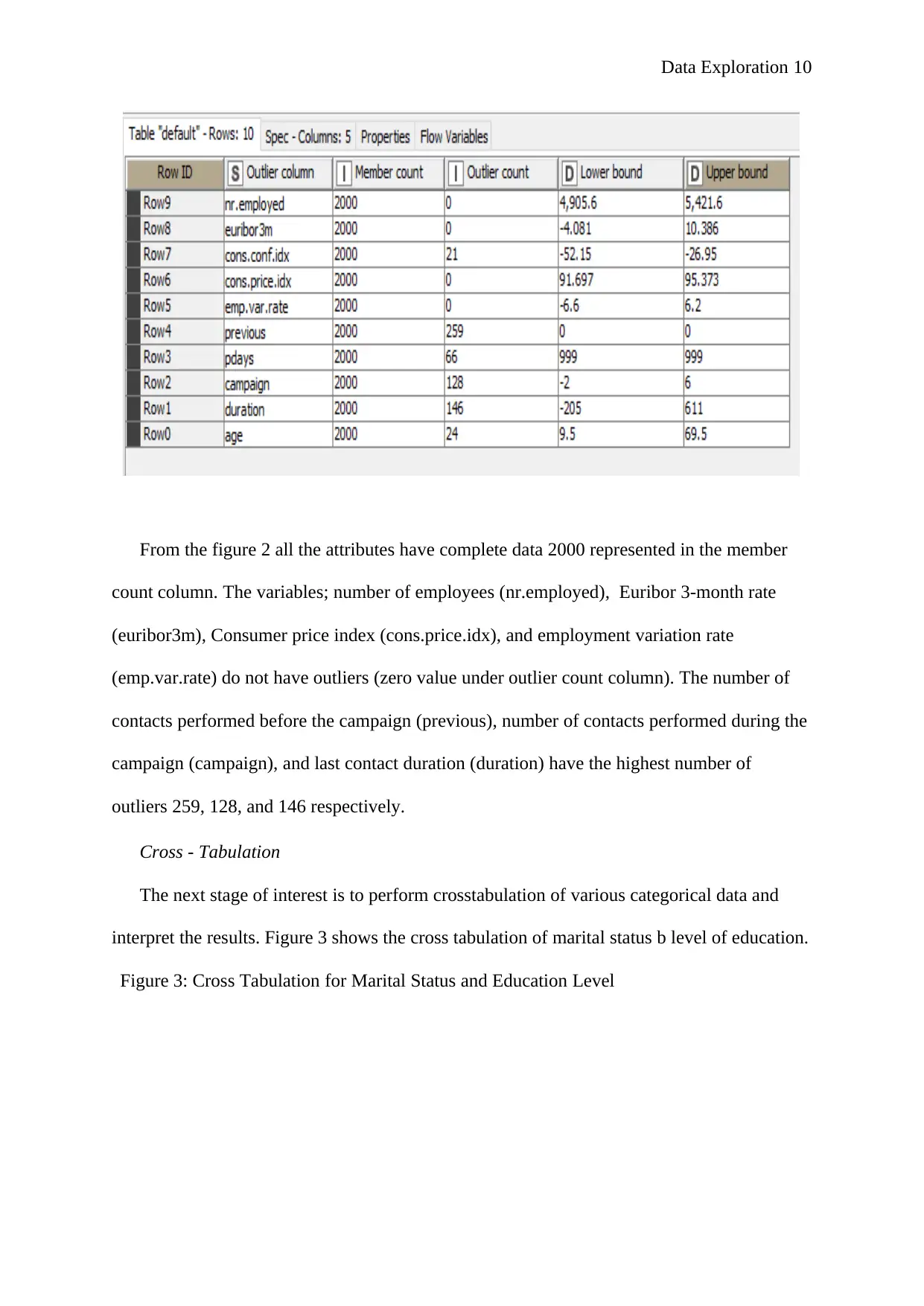
From the figure 2 all the attributes have complete data 2000 represented in the member
count column. The variables; number of employees (nr.employed), Euribor 3-month rate
(euribor3m), Consumer price index (cons.price.idx), and employment variation rate
(emp.var.rate) do not have outliers (zero value under outlier count column). The number of
contacts performed before the campaign (previous), number of contacts performed during the
campaign (campaign), and last contact duration (duration) have the highest number of
outliers 259, 128, and 146 respectively.
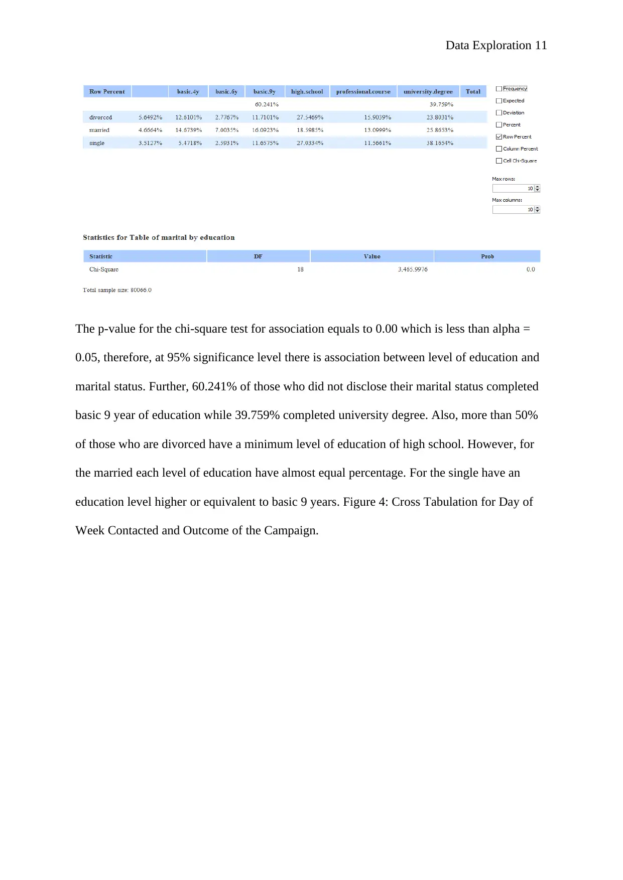
Cross - Tabulation
The next stage of interest is to perform crosstabulation of various categorical data and
interpret the results. Figure 3 shows the cross tabulation of marital status b level of education.
Figure 3: Cross Tabulation for Marital Status and Education Level

Data Exploration 11
The p-value for the chi-square test for association equals to 0.00 which is less than alpha =
0.05, therefore, at 95% significance level there is association between level of education and
marital status. Further, 60.241% of those who did not disclose their marital status completed
basic 9 year of education while 39.759% completed university degree. Also, more than 50%
of those who are divorced have a minimum level of education of high school. However, for
the married each level of education have almost equal percentage. For the single have an
education level higher or equivalent to basic 9 years. Figure 4: Cross Tabulation for Day of
Week Contacted and Outcome of the Campaign.

Data Exploration 12
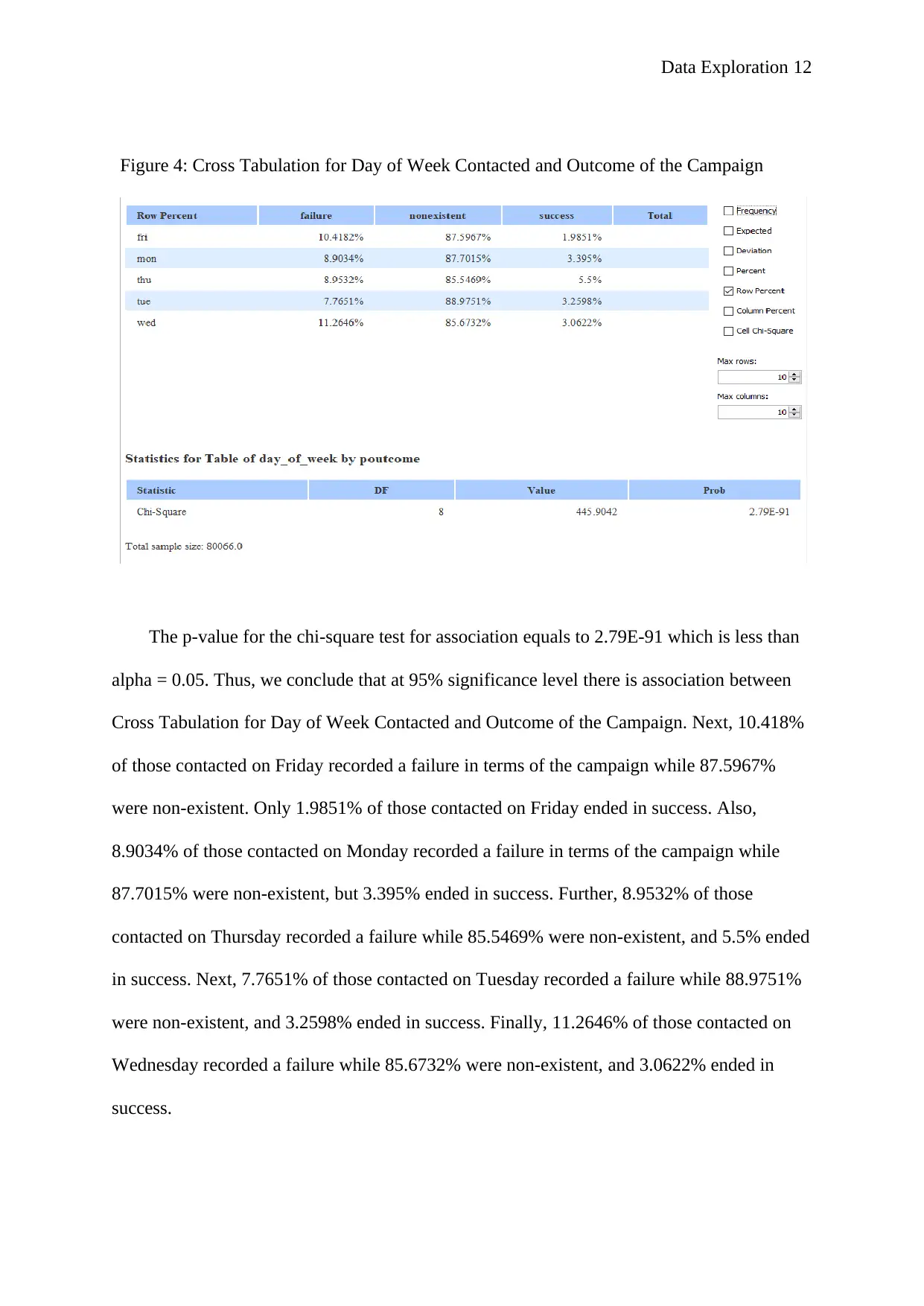
Figure 4: Cross Tabulation for Day of Week Contacted and Outcome of the Campaign
The p-value for the chi-square test for association equals to 2.79E-91 which is less than
alpha = 0.05. Thus, we conclude that at 95% significance level there is association between
Cross Tabulation for Day of Week Contacted and Outcome of the Campaign. Next, 10.418%
of those contacted on Friday recorded a failure in terms of the campaign while 87.5967%
were non-existent. Only 1.9851% of those contacted on Friday ended in success. Also,
8.9034% of those contacted on Monday recorded a failure in terms of the campaign while
87.7015% were non-existent, but 3.395% ended in success. Further, 8.9532% of those
contacted on Thursday recorded a failure while 85.5469% were non-existent, and 5.5% ended
in success. Next, 7.7651% of those contacted on Tuesday recorded a failure while 88.9751%
were non-existent, and 3.2598% ended in success. Finally, 11.2646% of those contacted on
Wednesday recorded a failure while 85.6732% were non-existent, and 3.0622% ended in
success.