Numeracy, Data & IT Assignment Solution - Detailed Analysis

This assignment solution covers a range of numeracy, data analysis, and IT skills, addressing problems related to proportions, percentages, calculations, and data interpretation. The solution demonstrates the application of mathematical concepts and the use of Excel for data organization and analysis. The assignment includes detailed explanations, step-by-step solutions, and the use of formulas for calculations, and the creation of charts. It explores topics such as Olympic medal analysis, highlighting data manipulation techniques, use of conditional formatting, ranking, and the application of formulas like SUM and AVERAGE. The document also includes the application of 'what if' analysis and demonstrates how to solve real-world problems using data-driven approaches. The assignment showcases proficiency in data handling, calculation, and presentation within the context of an IT environment.

Using Numeracy, Data & IT

Table of Contents
INTRODUCTION...........................................................................................................................3

TASK 1
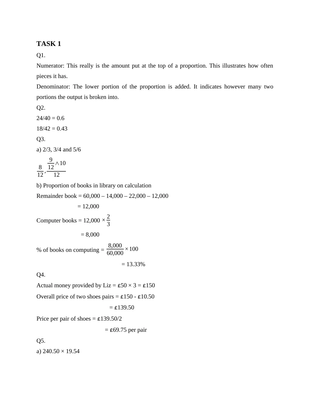
Q1.
Numerator: This really is the amount put at the top of a proportion. This illustrates how often
pieces it has.
Denominator: The lower portion of the proportion is added. It indicates however many two
portions the output is broken into.
Q2.
24/40 = 0.6
18/42 = 0.43
Q3.
a) 2/3, 3/4 and 5/6
8
12 ,
9
12 ∧10
12
b) Proportion of books in library on calculation
Remainder book = 60,000 – 14,000 – 22,000 – 12,000
= 12,000
Computer books = 12,000 × 2
3
= 8,000
% of books on computing = 8,000
60,000 ×100
= 13.33%
Q4.
Actual money provided by Liz = £50 × 3 = £150
Overall price of two shoes pairs = £150 - £10.50
= £139.50
Price per pair of shoes = £139.50/2
= £69.75 per pair
Q5.
a) 240.50 × 19.54

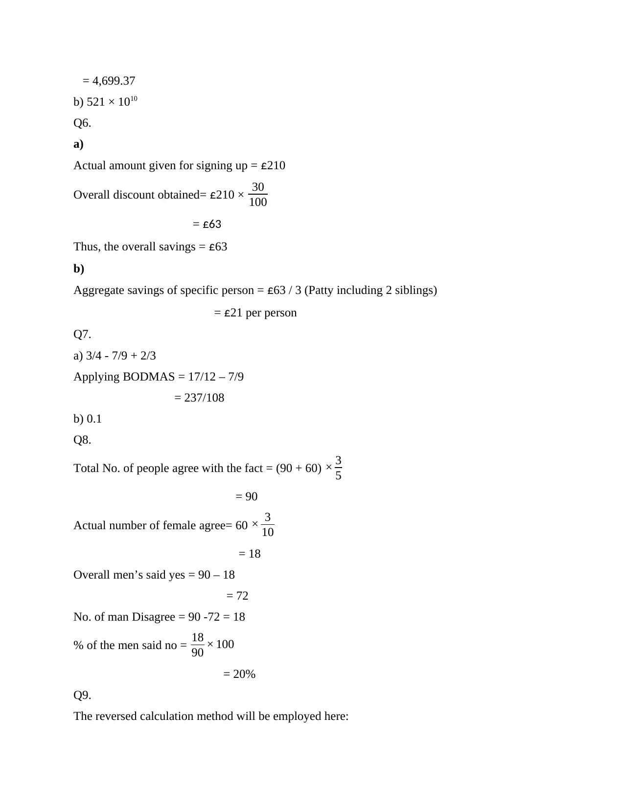
= 4,699.37
b) 521 × 1010
Q6.
a)
Actual amount given for signing up = £210
Overall discount obtained= £210 × 30
100
= £63
Thus, the overall savings = £63
b)
Aggregate savings of specific person = £63 / 3 (Patty including 2 siblings)
= £21 per person
Q7.
a) 3/4 - 7/9 + 2/3
Applying BODMAS = 17/12 – 7/9
= 237/108
b) 0.1
Q8.
Total No. of people agree with the fact = (90 + 60) × 3
5
= 90
Actual number of female agree= 60 × 3
10
= 18
Overall men’s said yes = 90 – 18
= 72
No. of man Disagree = 90 -72 = 18
% of the men said no = 18
90 × 100
= 20%
Q9.
The reversed calculation method will be employed here:

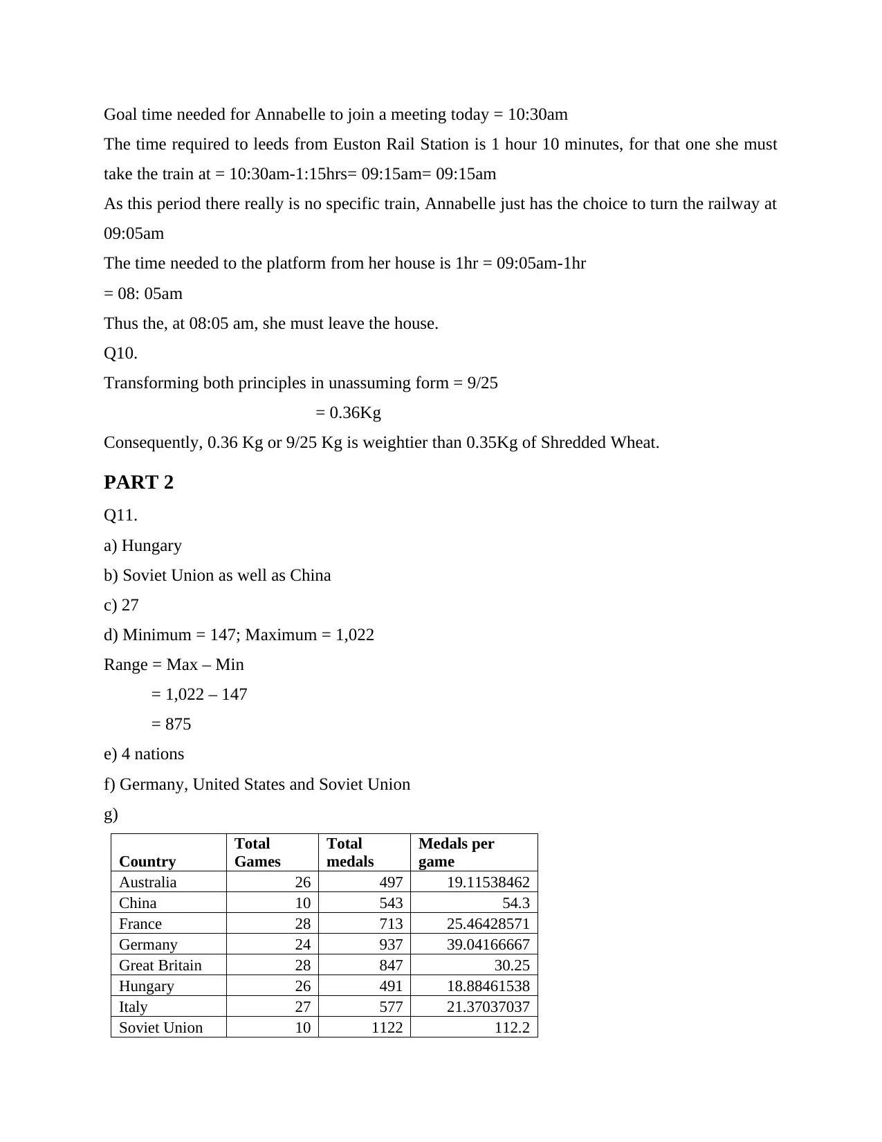
Goal time needed for Annabelle to join a meeting today = 10:30am
The time required to leeds from Euston Rail Station is 1 hour 10 minutes, for that one she must
take the train at = 10:30am-1:15hrs= 09:15am= 09:15am
As this period there really is no specific train, Annabelle just has the choice to turn the railway at
09:05am
The time needed to the platform from her house is 1hr = 09:05am-1hr
= 08: 05am
Thus the, at 08:05 am, she must leave the house.
Q10.
Transforming both principles in unassuming form = 9/25
= 0.36Kg
Consequently, 0.36 Kg or 9/25 Kg is weightier than 0.35Kg of Shredded Wheat.
PART 2
Q11.
a) Hungary
b) Soviet Union as well as China
c) 27
d) Minimum = 147; Maximum = 1,022
Range = Max – Min
= 1,022 – 147
= 875
e) 4 nations
f) Germany, United States and Soviet Union
g)
Country
Total
Games
Total
medals
Medals per
game
Australia 26 497 19.11538462
China 10 543 54.3
France 28 713 25.46428571
Germany 24 937 39.04166667
Great Britain 28 847 30.25
Hungary 26 491 18.88461538
Italy 27 577 21.37037037
Soviet Union 10 1122 112.2

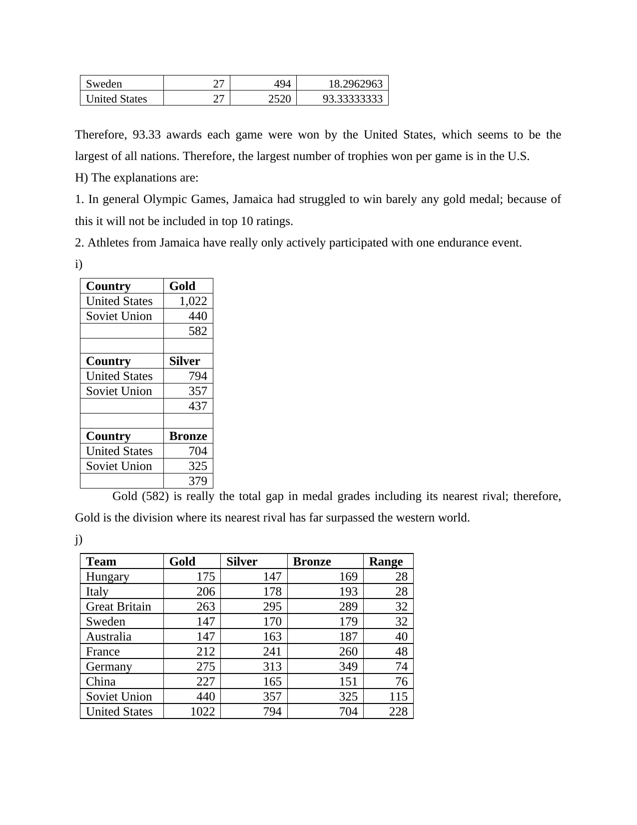
Sweden 27 494 18.2962963
United States 27 2520 93.33333333
Therefore, 93.33 awards each game were won by the United States, which seems to be the
largest of all nations. Therefore, the largest number of trophies won per game is in the U.S.
H) The explanations are:
1. In general Olympic Games, Jamaica had struggled to win barely any gold medal; because of
this it will not be included in top 10 ratings.
2. Athletes from Jamaica have really only actively participated with one endurance event.
i)
Country Gold
United States 1,022
Soviet Union 440
582
Country Silver
United States 794
Soviet Union 357
437
Country Bronze
United States 704
Soviet Union 325
379
Gold (582) is really the total gap in medal grades including its nearest rival; therefore,
Gold is the division where its nearest rival has far surpassed the western world.
j)
Team Gold Silver Bronze Range
Hungary 175 147 169 28
Italy 206 178 193 28
Great Britain 263 295 289 32
Sweden 147 170 179 32
Australia 147 163 187 40
France 212 241 260 48
Germany 275 313 349 74
China 227 165 151 76
Soviet Union 440 357 325 115
United States 1022 794 704 228

Part 3
Q12.
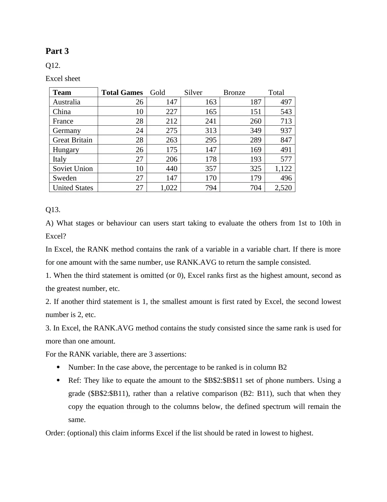
Excel sheet
Team Total Games Gold Silver Bronze Total
Australia 26 147 163 187 497
China 10 227 165 151 543
France 28 212 241 260 713
Germany 24 275 313 349 937
Great Britain 28 263 295 289 847
Hungary 26 175 147 169 491
Italy 27 206 178 193 577
Soviet Union 10 440 357 325 1,122
Sweden 27 147 170 179 496
United States 27 1,022 794 704 2,520
Q13.
A) What stages or behaviour can users start taking to evaluate the others from 1st to 10th in
Excel?
In Excel, the RANK method contains the rank of a variable in a variable chart. If there is more
for one amount with the same number, use RANK.AVG to return the sample consisted.
1. When the third statement is omitted (or 0), Excel ranks first as the highest amount, second as
the greatest number, etc.
2. If another third statement is 1, the smallest amount is first rated by Excel, the second lowest
number is 2, etc.
3. In Excel, the RANK.AVG method contains the study consisted since the same rank is used for
more than one amount.
For the RANK variable, there are 3 assertions:
 Number: In the case above, the percentage to be ranked is in column B2
 Ref: They like to equate the amount to the $B$2:$B$11 set of phone numbers. Using a
grade ($B$2:$B11), rather than a relative comparison (B2: B11), such that when they
copy the equation through to the columns below, the defined spectrum will remain the
same.
Order: (optional) this claim informs Excel if the list should be rated in lowest to highest.

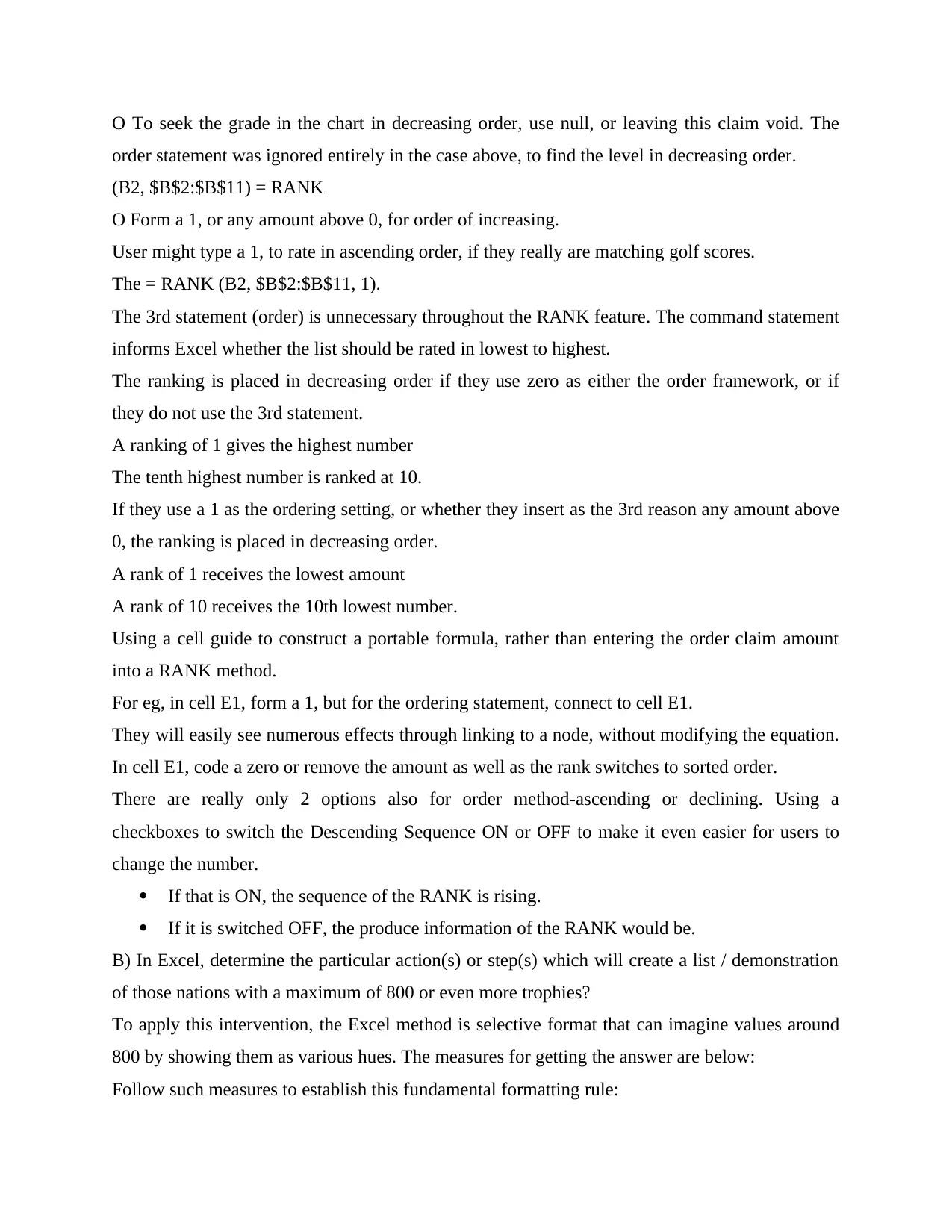
O To seek the grade in the chart in decreasing order, use null, or leaving this claim void. The
order statement was ignored entirely in the case above, to find the level in decreasing order.
(B2, $B$2:$B$11) = RANK
O Form a 1, or any amount above 0, for order of increasing.
User might type a 1, to rate in ascending order, if they really are matching golf scores.
The = RANK (B2, $B$2:$B$11, 1).
The 3rd statement (order) is unnecessary throughout the RANK feature. The command statement
informs Excel whether the list should be rated in lowest to highest.
The ranking is placed in decreasing order if they use zero as either the order framework, or if
they do not use the 3rd statement.
A ranking of 1 gives the highest number
The tenth highest number is ranked at 10.
If they use a 1 as the ordering setting, or whether they insert as the 3rd reason any amount above
0, the ranking is placed in decreasing order.
A rank of 1 receives the lowest amount
A rank of 10 receives the 10th lowest number.
Using a cell guide to construct a portable formula, rather than entering the order claim amount
into a RANK method.
For eg, in cell E1, form a 1, but for the ordering statement, connect to cell E1.
They will easily see numerous effects through linking to a node, without modifying the equation.
In cell E1, code a zero or remove the amount as well as the rank switches to sorted order.
There are really only 2 options also for order method-ascending or declining. Using a
checkboxes to switch the Descending Sequence ON or OFF to make it even easier for users to
change the number.
 If that is ON, the sequence of the RANK is rising.
 If it is switched OFF, the produce information of the RANK would be.
B) In Excel, determine the particular action(s) or step(s) which will create a list / demonstration
of those nations with a maximum of 800 or even more trophies?
To apply this intervention, the Excel method is selective format that can imagine values around
800 by showing them as various hues. The measures for getting the answer are below:
Follow such measures to establish this fundamental formatting rule:

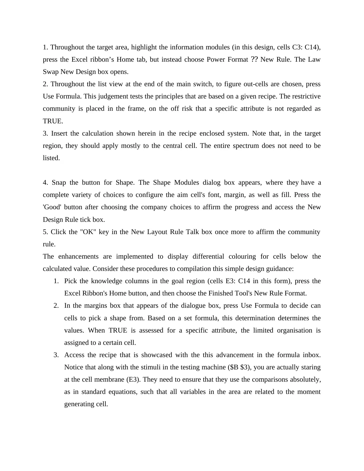
1. Throughout the target area, highlight the information modules (in this design, cells C3: C14),
press the Excel ribbon’s Home tab, but instead choose Power Format New Rule. The Law⁇
Swap New Design box opens.
2. Throughout the list view at the end of the main switch, to figure out-cells are chosen, press
Use Formula. This judgement tests the principles that are based on a given recipe. The restrictive
community is placed in the frame, on the off risk that a specific attribute is not regarded as
TRUE.
3. Insert the calculation shown herein in the recipe enclosed system. Note that, in the target
region, they should apply mostly to the central cell. The entire spectrum does not need to be
listed.
4. Snap the button for Shape. The Shape Modules dialog box appears, where they have a
complete variety of choices to configure the aim cell's font, margin, as well as fill. Press the
'Good' button after choosing the company choices to affirm the progress and access the New
Design Rule tick box.
5. Click the "OK" key in the New Layout Rule Talk box once more to affirm the community
rule.
The enhancements are implemented to display differential colouring for cells below the
calculated value. Consider these procedures to compilation this simple design guidance:
1. Pick the knowledge columns in the goal region (cells E3: C14 in this form), press the
Excel Ribbon's Home button, and then choose the Finished Tool's New Rule Format.
2. In the margins box that appears of the dialogue box, press Use Formula to decide can
cells to pick a shape from. Based on a set formula, this determination determines the
values. When TRUE is assessed for a specific attribute, the limited organisation is
assigned to a certain cell.
3. Access the recipe that is showcased with the this advancement in the formula inbox.
Notice that along with the stimuli in the testing machine ($B $3), you are actually staring
at the cell membrane (E3). They need to ensure that they use the comparisons absolutely,
as in standard equations, such that all variables in the area are related to the moment
generating cell.

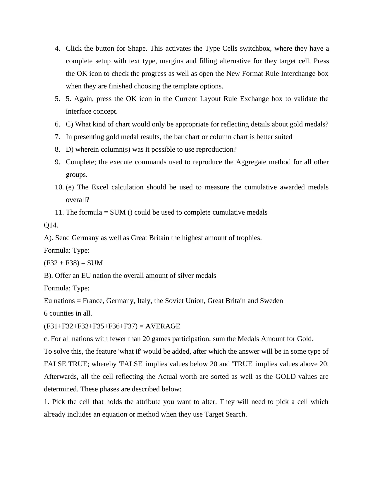
4. Click the button for Shape. This activates the Type Cells switchbox, where they have a
complete setup with text type, margins and filling alternative for they target cell. Press
the OK icon to check the progress as well as open the New Format Rule Interchange box
when they are finished choosing the template options.
5. 5. Again, press the OK icon in the Current Layout Rule Exchange box to validate the
interface concept.
6. C) What kind of chart would only be appropriate for reflecting details about gold medals?
7. In presenting gold medal results, the bar chart or column chart is better suited
8. D) wherein column(s) was it possible to use reproduction?
9. Complete; the execute commands used to reproduce the Aggregate method for all other
groups.
10. (e) The Excel calculation should be used to measure the cumulative awarded medals
overall?
11. The formula = SUM () could be used to complete cumulative medals
Q14.
A). Send Germany as well as Great Britain the highest amount of trophies.
Formula: Type:
(F32 + F38) = SUM
B). Offer an EU nation the overall amount of silver medals
Formula: Type:
Eu nations = France, Germany, Italy, the Soviet Union, Great Britain and Sweden
6 counties in all.
(F31+F32+F33+F35+F36+F37) = AVERAGE
c. For all nations with fewer than 20 games participation, sum the Medals Amount for Gold.
To solve this, the feature 'what if' would be added, after which the answer will be in some type of
FALSE TRUE; whereby 'FALSE' implies values below 20 and 'TRUE' implies values above 20.
Afterwards, all the cell reflecting the Actual worth are sorted as well as the GOLD values are
determined. These phases are described below:
1. Pick the cell that holds the attribute you want to alter. They will need to pick a cell which
already includes an equation or method when they use Target Search.

2. Click the What-If Review order on the Data tab, but instead pick Target again from drop-down
menu.
3. With 3 areas, a dialog box appears:
Set cell: This is the cell that holds the outcome that you seek. In our situation, cell B7 has already
been picked.
To value: This really is the outcome that is expected. There will be entering 70 in certain case,
because they need to pay at least that to practice regularly.
By altering the cell: This really is the cell where even the response is placed by score Seek. In the
example, user will select cell B6 because we want to determine the grade we need to earn on the
final assignment.
4.
If Objective Seek is able to make it work, the dialogue box will inform the user. Only press OK.
5.
In the stated unit, the outcome will occur. In our case, Target Seek determined that in order to ob
tain a pass mark, they will have to win at least 90 mostly on final project.
D). To identify 'Italy' and even the related Medals Complete, browse the index (the entire
spreadsheet). The design of VLOOKUP is applied here; VLOOKUP standing for "easy check."
In Excel, this implies looking for best deal in a database, use spreadsheet segments: but as the
primary source for the quest, including specific identifiers throughout these divisions. If they
review the results, anywhere it is identified, it should be registered explicitly.
1. Define a row of cells that user want to populate with new info.
2. Choose 'Feature' (Fx) > VLOOKUP and paste this equation into the cell they highlighted.
3. Input the lookup attribute for which user want new information to be retrieved.
4. Join a spreadsheet tables list where even the required data is stored.
5. Input the column amount of the information they wish to return from Excel.
6. To identify the correct or estimated matching of the search value, enter any selection lookup.
7. Select 'Right' (or 'Enter') and the new row will be filled in.
Q15.
A) By each category of medal, measure the median number of medals, specifying the calculation
you will use to estimate the median for the gold medals.

• The median is determined as the middle element in the category whenever the overall amount
of provided figures is odd.
The median is determined as the sum of the two figures in the centre while the overall number of
provided items is even.
• Ignore columns that potentially contain, maximum quantity, or no value.
• Numbers may be given as numbers, sets, called sets, or references to cells containing numerical
values. Up to 255 number could be supplied.
There is no built-in means of adding parameters to the MEDIAN feature. Provided a scope, the
MEDIAN (middle) number within this range would be returned. They use the IF feature within
MEDIAN to 'sort' values in order to add parameters.
So, firstly, variables will be reordered and median would be listed for 5th as well as 6th position.
Gold Median:
219.5
Silver Median:
209.5
Bronze median:
206.5
b) Calculate the mean number of medals for each of the 3 medal types, stating the formula
you would use for determining the mean for the bronze medals.
Mean:
Gold = 311; Silver = 282 and Bronze = 281.
FORMULA;
Mean is indeed a system of principles its nothing but a median. Therefore, the mean of
Bronze models (= AVERAGE (E29: E38)) will be defined by an average feature.
c) Calculate the standard deviation of the total medals awarded to each country (column F)
using the formula below.
Standard Deviation σ = 288.60926
Variance σ2 = 83295.306
Count n = 12

Mean x¯ = 478.83333
Sum of Squares SS = 999543.67
σ = √ ∑ ( x −u ) 2
N
σ = √ 999543.67
12
= √83295.306
= 288.60926
D) Address the utility of a standard deviation in such a testing set that use the given chart as a
reference.
The most widely used variance proportion in an observable procedure is point difference as
averaging is being used to calculate focal bias. It predicts the normal circulation, as these lines
do. Due to the near links to the means, if the mean has an unassisted aspect of the attention
deflection, a regular movement may have a major impact.
Exclusions that may normally be applied in the wake of the specific deviation are often protected
by the standard deviation. In this context, a fair suggestion that there really are variations is
universal bias. This renders natural motion, without anomalies, a very useful component of the
propagation for correct ratio.
Standard deviation also is beneficial when compared with the rest of two different normal size
pieces of information. For the normal minor distortion, there is less spreading of predictions
around knowledge collection, and therefore the results are larger or lesser in the most portion. An
object chosen from an instance shows which has a lower mean variance for a greater potential to
be similar to the average is indeed an item with a higher average variance with an instance
shows.
The further common the results, the stronger the common prejudice, in most situations. For
instance, note that they need to isolate two unique confirmatory testing requirements from either
a group of 30 students, the key assessment has subject to different regulations from 31% to 98%,

ranging from 82% to 93%. For these modifications, the cumulative preference towards the key
test's effects will be higher.
16.
A)
Australia
China
France
Germany
Great Britain
Hungary
Italy
Soviet Union
Sweden
United States
0
500
1000
1500
2000
2500
3000
Total
B)
6% 6%
8%
11%
10%
6%7%
13%
6%
29%
Total
Australia
China
France
Germany
Great Britain
Hungary
Italy
Soviet Union
Sweden
United States