Comprehensive Solution for MIT4204 Data Mining Assignment

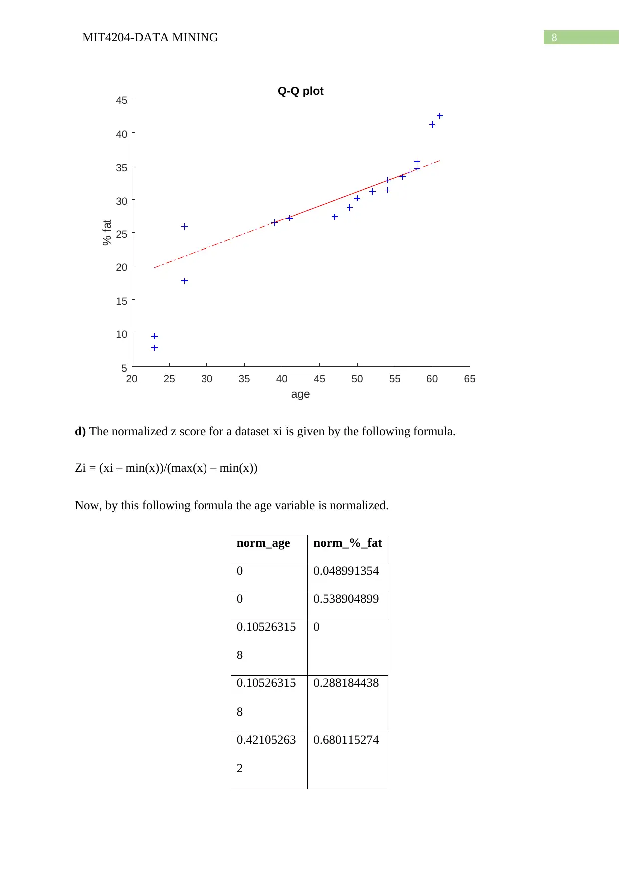
This document provides a detailed solution to a data mining assignment, covering a wide range of topics. It begins with statistical analysis, including calculations of mean, median, mode, midrange, quartiles, and the five-number summary, along with the creation of a boxplot and explanation of quantile plots. The solution then delves into distributive, algebraic, and holistic measures, and addresses methods for handling missing data. Further, it explores data smoothing techniques such as bin means, and discusses outliers and different smoothing methods. The assignment continues with an analysis of a dataset involving age and %fat, including calculations of mean, standard deviation, boxplots, scatter plots, and Q-Q plots, as well as normalization and correlation analysis. The solution also covers data integration approaches, schema types for data warehouses (star, snowflake, fact constellation), OLAP operations, and data warehouse modeling, including SQL queries. Finally, the document addresses data refresh, cleaning, and transformation processes, as well as the differences between data marts, enterprise warehouses, and virtual warehouses. Desklib offers this and many more past papers and solved assignments for students to excel in their studies.

0MIT4204-DATA MINING
MIT4204-DATA MINING
Name of the Student
Name of the University
Author Note

1MIT4204-DATA MINING
Question 1:
The given dataset of attribute age is
13, 15, 16, 16, 19, 20, 20, 21, 22, 22, 25, 25, 25, 25, 30, 33, 33, 35, 35, 35, 35, 36, 40, 45, 46,
52, 70.
a) The mean of the attribute age is calculated by summing all the values and then dividing the
sum by number of values. This is calculated in excel as given below.
Hence, the mean of the data as calculated in excel is
Mean = 29.96296
Median = 25
b) The mode of the data is given by,
The number which has the highest frequency in the data set.
Now, two numbers 25 and 35 are in the dataset for 4 times which is highest number of
occurrence. Hence, the data is bimodal as there are two modes which are 25 and 35.
c) The midrange of the data set is given by,
Middle range = (range/2) = (maximum – minimum)/2 = 28.5.
Now, the midrange value = minimum + (range/2) = 28.5 + 13 = 41.5.
d) The first quartile is the mid-value of the minimum and median value and the third quartile
is the mid-value of the median and the maximum value.
Q1 = 20 and Q3 = 35.
e) The five-number summary of data is given below.
Minimum 13

2MIT4204-DATA MINING
Q1 20
Median 25
Q3 35
Maximum 70
Hence, 5 number summary is 13,20,25,35, 70.
The boxplot is shown below.
70
60
50
40
30
20
10
Values
Boxplot of Values
g) In the quantile plot the quantiles of a set of values are displayed. The sample quantiles are
in Y axis and fraction of sample they correspond are in the x axis.
In the Quantile-quantile (Q-Q) plot the quantiles of two sets of data are compared. The
comparison is more than just comparing the mean and median, the shapes of the two datasets
are also compared.

3MIT4204-DATA MINING
Question 2:
The distributive measures are those measures which gives the same results when applying on
the whole dataset and in the subgroups of dataset. For example, the functions like count, sum,
min and max are distributive measures as measure of the whole dataset is obtained by just
summing up the values for the subgroups. The Algebraic measure are the measures which can
be computed for the whole dataset by using an algebraic function of n arguments (n is
positive integers) in the subgroups. Average is an algebraic measure as average = sum /
count. If for some measure there exists no algebraic function which can compute the measure
of total dataset by using the measures in subgroups then those are the holistic measures. Some
examples of the holistic measures are mode, median and rank.
Question 3:
Missing values in a dataset is common for real world scenarios as all the sample observations
are complete in very rare cases. Now, common practise to deal with missing values is to
remove those missing pairs and do the analysis with the rest values which are complete. Now,
this gives good accuracy when the missing values are within 5% of the sample size.
However, when the missing values are very large then the case is discarded and the data
collection is performed again. In case of univariate analysis an intuitive guess can be applied
if there is less number of missing values to have sufficient amount of accuracy in the
analysis.
Question 4:
The given dataset is
13, 15, 16, 16, 19, 20, 20, 21, 22, 22, 25, 25, 25, 25, 30, 33, 33, 35, 35, 35, 35, 36, 40, 45, 46,
52, 70.

4MIT4204-DATA MINING
a) Now, in the smoothing by means technique the whole dataset is divided into several parts
with number of values in a part equal to the bin depth. Then the average of the values in a
part is calculated and all the values in that part is replaced with the average.
Now, bin depth = 3.
Hence, smoothing by bin means:
bin 1 = 14.66666667, 14.66666667, 14.66666667
bin 2 = 18.33333333, 18.33333333, 18.33333333
bin 3 = 21, 21, 21
bin 4 = 24, 24, 24
bin 5 = 26.66666667, 26.66666667, 26.66666667
bin 6 = 33.66666667, 33.66666667, 33.66666667
bin 7 = 35, 35, 35
bin 8 = 40.33333333, 40.33333333, 40.33333333
bin 9 = 56, 56, 56.
Smoothing data by means will move the noises in the data and a smooth curve can be found
for the given data.
b) The outliers in a data set are the points which are over Q3 + 1.5*IQR and below Q1 –
1.5*IQR.
Where, Q1 = 1st quartile, Q3 = 3rd quartile
IQR = Q3 – Q1

5MIT4204-DATA MINING
c) The other types of data smoothing are smoothing by equal frequency and smoothing by bin
boundaries.
Different issues in data integration are varied information, lack of manpower, storeroom
competence shortage and awful information.
Question 5:
Age % Fat
23 9.5
23 26.5
27 7.8
27 17.8
39 31.4
41 25.9
47 27.4
49 27.2
50 31.2
52 34.6
54 42.5
54 28.8
56 33.4
57 30.2
58 34.1
58 32.9
60 41.2
61 35.7
a) The mean and standard deviation of age and %fat is calculated in excel as given below.

6MIT4204-DATA MINING
mean age 46.44444
median age 51
std age 13.21862
mean % fat 28.78333
std %fat 9.254395
median % fat 30.7
b) The boxplots of age and %fat are constructed using Minitab as given below.
% fatage
60
50
40
30
20
10
0
Data
Boxplot of age, % fat
c) The scatter plot is constructed where the age is considered as independent variable(x axis)
and the %fat is considered as dependent variable (y axis).

7MIT4204-DATA MINING
20 25 30 35 40 45 50 55 60 65
0
5
10
15
20
25
30
35
40
45
Scatter plot
age (in years)
% fat
The q-q plot of age and % fat is constructed in MATLAB and given below.
Matlab code:
>> age = [23 23 27 27 39 41 47 49 50 52 54 54 56
57 58 58 60 61];
>> percent_fat = [9.5 26.5 7.8 17.8 31.4 25.9 27.4 27.2 31.2 34.6
42.5 28.8 33.4 30.2 34.1 32.9 41.2 35.7];
>> qqplot(age,percent_fat)
>> xlabel('age'); ylabel('% fat')
>> title('Q-Q plot')

8MIT4204-DATA MINING
20 25 30 35 40 45 50 55 60 65
age
5
10
15
20
25
30
35
40
45
% fat
Q-Q plot
d) The normalized z score for a dataset xi is given by the following formula.
Zi = (xi – min(x))/(max(x) – min(x))
Now, by this following formula the age variable is normalized.
norm_age norm_%_fat
0 0.048991354
0 0.538904899
0.10526315
8
0
0.10526315
8
0.288184438
0.42105263
2
0.680115274

9MIT4204-DATA MINING
0.47368421
1
0.521613833
0.63157894
7
0.564841499
0.68421052
6
0.55907781
0.71052631
6
0.674351585
0.76315789
5
0.772334294
0.81578947
4
1
0.81578947
4
0.60518732
0.86842105
3
0.737752161
0.89473684
2
0.645533141
0.92105263
2
0.757925072
0.92105263
2
0.723342939
0.97368421
1
0.962536023
1 0.804034582

10MIT4204-DATA MINING
e) The Pearson’s correlation coefficient is calculated by the correl function in excel.
Correl(age,%fat) = 0.817618796.
Hence, the two variables are positively correlated. This is also evident from the scatterplot of
the two variables.
Question 6:
The two approaches for the integration of different heterogeneous sources of information are
update driven approach and the query driven approach. Update driven approach is the most
popular and efficient method as the information is copied, process and restructured from
many heterogeneous sources before doing the data analysis. Thus no interface is required for
query processing in update driven approach. Thus Update driven approach is preferred in
many industries for its high performance and efficient solution. The query driven approach is
used for building wrappers and the integrators on the top of the heterogeneous databases.
This is basically needed when the query needs are unknown.
Question 7:
a)
Star schema Snowflake Schema Fact Constellation
There is only one central
fact table and each
dimension has one table.
There is only one central
fact table and each
dimension has one table.
Dimension tables are shared
by multiple fact tables.
The hierarchies are not
directly captured.
Vary form Star schema. Viewed as collection of stars
and known as galaxy
schema.
Each of the fact points are in The dimension tables are The schema is for

11MIT4204-DATA MINING
one tuple in a single
dimension with additional
attributes.
normalized and then split
into additional tables.
sophisticated applications.
b) Data refresh is a method where entire data solution is re-built in several large batches from
scratch. The initial load of batch processing code is used for refreshing data.
Data cleaning is basically a process of detecting and then correcting corrupted data records
from a table or a database and the identification of incorrect, incomplete or any irrelevant
parts of data. Then these parts of data are either replaced or modified or deleted. These
corrupted part of data are known as dirty or coarse data.
In data transformation process data is transformed to a form which is suitable for applying the
data mining process. Some of the data transformation strategies are smoothing, aggregation,
generalization, normalization, attribute construction. By smoothing noise is removed from
data. In aggregation process the summary operations are applied to data. In the process of
generalization the low levels of data are efficiently replaced with high level of data by the
hierarchy climbing process. Normalization is a process of scaling data such that it falls under
the range 0 to 1. In case of attribute reconstruction new types of attributes are made from
attributes which are available.
c) The enterprise warehouse is particularly a system which is used for data analysis and
reporting and it is the most fundamental component of the business. It is the central
repositories of the integrated data extracted from one or more disparate source.
The data mart is basically an access pattern or a structure that is built for particularly data
warehouse environments for retrieving the data that is more client faced. It is basically a
subset of a large data warehouse and directed to a particular team or business line.

12MIT4204-DATA MINING
A virtual warehouse is basically a term which is used for the data warehousing and it is a
business database. The particular data found in the virtual warehouse is a copy of data from
multiple sources.
Question 8:
a) The most popular classes of schema for data warehouse modelling are
i) Star schema: This is made with central fact table and dimension tables. The two sets of
columns in the fact table of this schema contain foreign keys which are known as the primary
keys for the dimension tables and measure of facts respecotively.
ii) Snowflake schema: This is very similar to the star schema having just two levels of the
dimension tables. The tables of dimension are normalized and then split in two by using
relevant data.
iii) Fact constellation: This is made using two interconnected Fact tables associated with
dimension tables.
b) Now, the star schema diagram for data house as given in the question is given below.

13MIT4204-DATA MINING
c) The specific operations in order is given below.
1. Rolling up from day then to month and then to year
2. Slice year = “2004”
3. Individual patient to all patient roll up
4. Patient slice = “all”
5. Obtaining the list of total collected fee by every doctor in the year 2004.
d) SQL query assuming the data is stored in a relational database using star schema is given
below.
SQL
Select doctor, Sum(charge)
From fee
Where year = 2004
Group by doctor
Question 9:
a) The snowflake schema diagram for data warehousing is shown below.

14MIT4204-DATA MINING
b) Starting with the base cuboid, the specific OLAP operations that must be performed for
listing the average operations are given below.
[student, course, semester, instructor]
1. from course_key to major roll-up on course
2. from student_key to university roll-up on student.
3. Student in department = “CS” and university = “Big University” dicing on course.
4. from University to student name drilling down on student
c) As each dimension has 5 level and each level there are 4 cuboids hence the cube will
contain 5^4 = 625 cuboids.
Question 10:
a) The star schema diagram for the given data warehouse is the following.

15MIT4204-DATA MINING
b) The specific OLAP operations are given below.
1. date_id to year roll up on date
2. game_id to all roll up on game
3. location_id to location_name roll up on location
4. spectator_id to status roll up on spectator
5. Location name = “GM_Place”, year = 2004 and Dice status = “students”
c) The Bitmap indexing is very useful technique in data warehousing. This technique is
beneficial in low-cardinally domains. Now, as an example when the dimension location is
indexed by bitmap then joining, comparison and aggregation operations over the locations are
reduced in bit arithmetic and thus the processing time is reduced.
Question 11:
a) The ROLAP technique is basically consist of intermediate servers in between the back end
and front end server and thus it uses a relational or extended-relational DBMS for storing and

16MIT4204-DATA MINING
managing the warehouse data. The MOLAP implementation has servers that supports the
multidimensional view of the data by the multidimensional storage engines. The HOLAP is
the combination of ROLAP and MOLAP and thus large volume of detailed data can be stored
in HOLAP.
b) Using ROLAP the data warehouse generation is implemented with the use of relational
and extended-relational DBMS by the use of fact tables.
Question 12:
a) The particular structure of the data cube is for supporting the preference that would be for
using partial level of materialization or to select computation cuboids. The total storage space
can be reduced when only the proper subsets among the whole set of cuboids are calculated.
This also reduces the response time.
b) As the user’s choice is to drill within one or two dimensions, the feature can be supported
with the computation of the required cuboids those are on the fly. This particular feature is
not needed by the user for many times and thus the extra time required for computation of
one or two dimensions those are on the fly can be easily accepted.
Question 13:
The information processing have the queries for finding and reporting information by the use
of crosstabs, graphs, charts and tables. The technique of analytical processing use different
types of OLAP operations like slice and dice, drill down, roll up and historical data pivoting
for the case of analysis of multidimensional warehouse data. The data mining uses the
discovery of the knowledge for finding patterns which are hidden and associations,
construction of analytical models, performance of prediction and classification.

17MIT4204-DATA MINING
On-line selection of the data mining functions basically allows the users who do not know the
different knowledge that should be mined by the flexibility for selecting the desired functions
of data mining and then data mining tasks are dramatically swapped.
Question 14:
a) The maximum number of cells possible in the cuboid which is regarded as base is p^n.
This the largest number of distinct tuples that can be formed from p distinct numbers in every
dimension.
b) p tuples are needed for containing p distinct values in each of the dimensions. Hence,
minimum number of cells possible in the base cuboid is p.
c) Additionally, a ∗ can also be chosen other than the p distinct values for
each dimension. Thus maximum number of cells possible for n
dimensions is (p+1)^n.
d) The minimum cell number is the number when there are p cells in
every cuboid other than the apex that has a single cell.
Question 15:
a) The complete lattice structure of the cube is given below.

18MIT4204-DATA MINING
b) The total size of the computed cube is calculated below.
All = 1
A = 1,000,000, B = 100 and C = 1000. Hence, subtotal = 1,001,100.
AB = 100,000,000, BC = 100,000, AC = 1,000,000,000 and hence the subtotal =
1,100,100,000.
ABC = 100,000,000,000.
Hence, total size in bytes = 101,101,101,101 ×4 bytes = 404,404,404,404 bytes.
c) The least amount of space is required in computation order B-C-A. The diagram is shown
below.

19MIT4204-DATA MINING
The total space required = 100 * 1000 + 1,000,000 * 10 + 100*10000 = 20,100,000 =
80,400,000 bytes.
Question 16:
a) The OLAP operations are listed in a sequence.
i. Level of category and dice on “business” roll up on traveller.
ii. In the level of city and on dice “L.A” on departure.
iii. In the level of “ANY” roll up on the “departure_time”
iv. In the level of “ANY” roll up on the arrival.
v. In the level of “ANY” roll-up on the arrival time
vi. In the level of company and dice on “AA” roll up on flight.
vii. In the level of individual drill down on traveller.
viii. In the level of month drill down on the departure-time.

20MIT4204-DATA MINING
b) The two constraints are min_sup = 10 and avg_fare > 500. When using the iceberg cubing
algorithm like BUC we get avg_fare > 500. Now, as avg_fare is anti-monotonic, hence, this
should be converted to a top-k-avg or avg^10(fare) > 500. Now for pruning the computation
of the cube binning is added to min_sup.
Question 17:
a) The itemsets that are frequent by using Apriori and FP-growth are given below.
Apriori:
The FP-growth tree is shown below

21MIT4204-DATA MINING
The FP growth table is given below.
item Conditional pattern base Conditional
tree
Frequent pattern
y {{k,e,m,o:1},{k,e,o:1},{k,m:1}} k:3 {k,y:3}
o {{k,e,m:1},{k,e:2}} k:3,e:3 {k,o:3},{e,o:3},{k,e,o:3}
m {{k,e:2},{k:1}} k:3 {k,m:3}
e {{k:4}} k:4 {k,e:4}
Apriori does many scans in the database, however the FP-growth can build a FP-Tree with
just only one scan. Hence, FP-growth is more time efficient than Apriori. Apriori needs to
generate candidates and those generations are expensive but there is no candidate generation
in FP-growth technique.
Question 18:
a) The rule template for granularity of item_category is
∀X ∈ transaction, buys(X,item1) ∧ buys(X,item2) => buys(X,item3)
[s,c]

22MIT4204-DATA MINING
The frequent k-itemset is listed for the maximum value of k and with
confidence and support c and s respectively all of strong association rules
are listed.
According the question
k = 3 and 3-items are {Bread, Milk, Cheese}.
Now, the rules are
Bread ∧ Cheese => Milk, [75% and 100%]
Cheese ∧ Milk => Bread, [75% and 100%]
Cheese => Milk ∧ Bread, [75% and 100%]
b) The rule template for the brand-item-category is given below,
∀X ∈ customer, buys(X, item1) ∧ buys(X, item2) => buys(X, item3)
Listing all of the frequent k-itemset for finding the maximum k value.
Here, k= 3 and itemset = {(Wonder-bread, Dairyland-milk, Tasty-Pie),
(Wonder-Bread, Sunset-Milk, Dairyland-Cheese)}