Data Mining and Visualization Business Case Analysis Solution - [Date]

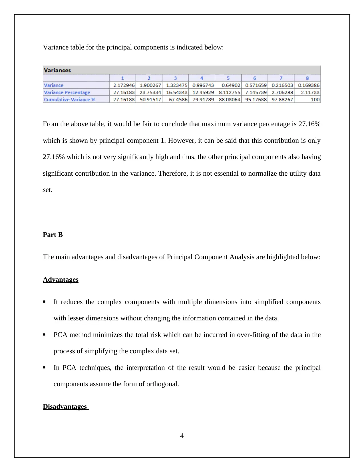
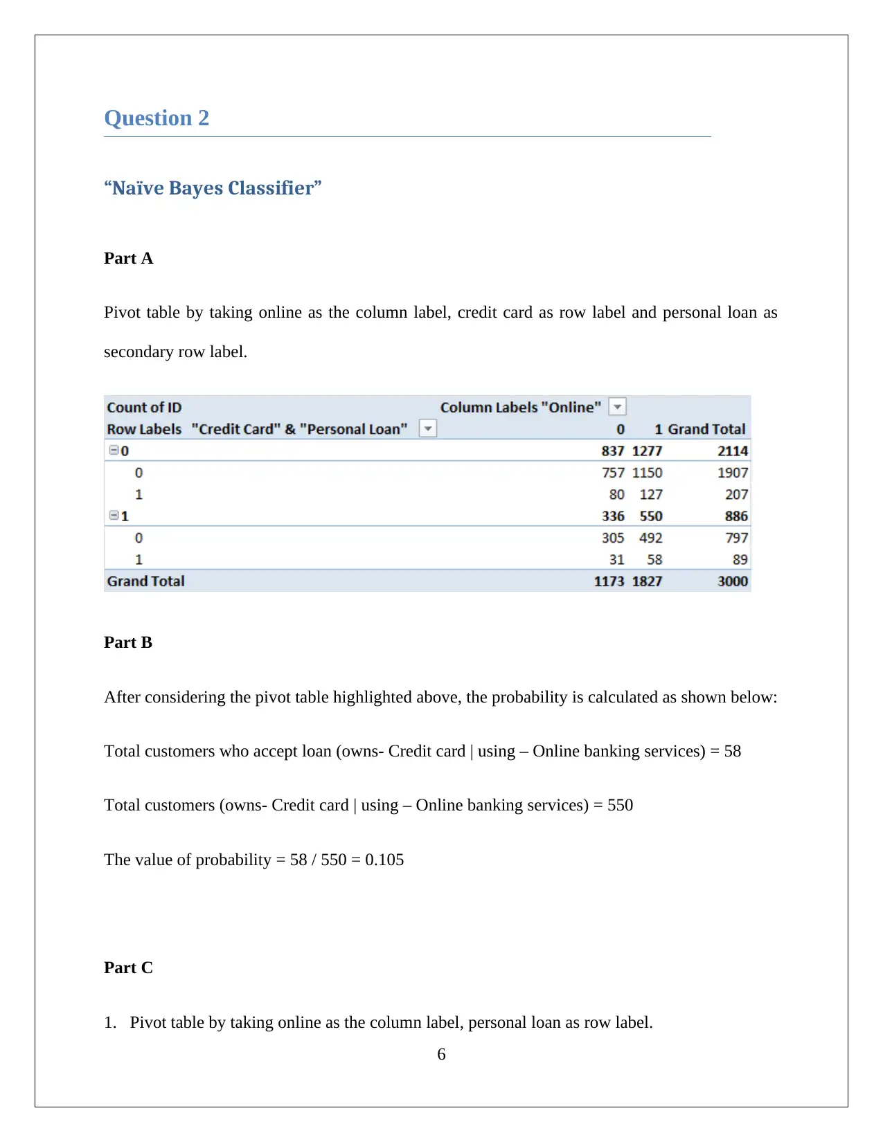
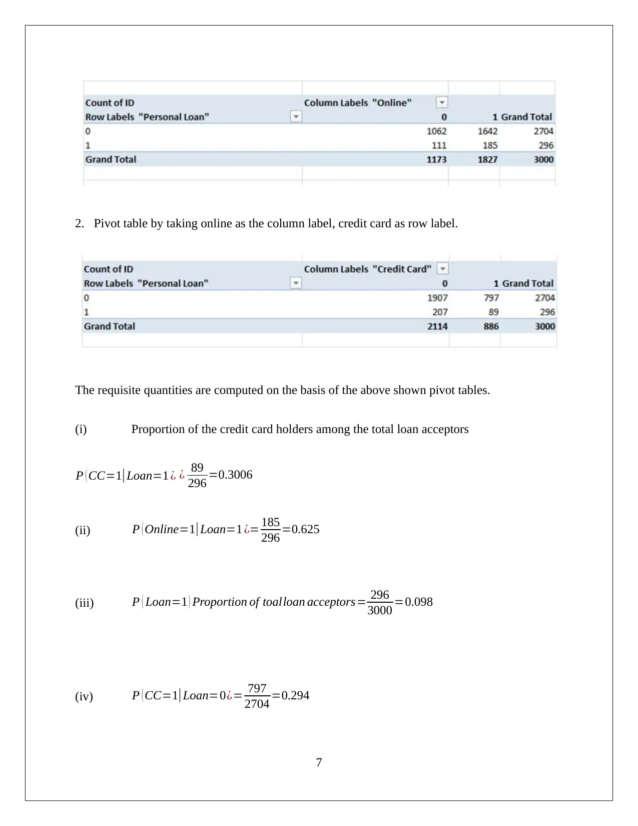
This assignment solution provides a detailed analysis of a business case in Data Mining and Visualization. It covers two main questions: the first focuses on Dimension Reduction using Principal Component Analysis (PCA) applied to a utilities dataset, including comments on PCA results, identification of...Read More

Data Mining and Visualization
Business Case Analysis 1
[Pick the date]
Student Id

Question 1
“Dimension Reduction”
Part A
Utility data set
Principal component analysis (PCA) for the utilities data set is performed in Excel by using
XLMiner tool and is shown below:
1

Comments on PCA result:
 The primary six principal components (1, 2, 3, 4, 5 and 6) would be the key principal
components. This is because nearly 95% of variances have been discussed by these principal
components.
 Therefore, the output from XLMiner would comprise only six primary principal components
and is given below.
2

 The next step is to determine the principal components and the significant features that would
be shown below.
 After considering the variance table and their respective contribution in total variance, it can
be cited that the central features would be x2, x6 and x7 (Rate of return on capital, sales,
percent nuclear).
Data Normalization: Data normalization would be required when a single variable has
contributed significant high % to the total variances. In the present case scenario, it is essential
to determine the whether any particular variable is showing significantly high contribution to the
total variation or not.
3

Variance table for the principal components is indicated below:
From the above table, it would be fair to conclude that maximum variance percentage is 27.16%
which is shown by principal component 1. However, it can be said that this contribution is only
27.16% which is not very significantly high and thus, the other principal components also having
significant contribution in the variance. Therefore, it is not essential to normalize the utility data
set.
Part B
The main advantages and disadvantages of Principal Component Analysis are highlighted below:
Advantages
 It reduces the complex components with multiple dimensions into simplified components
with lesser dimensions without changing the information contained in the data.
 PCA method minimizes the total risk which can be incurred in over-fitting of the data in the
process of simplifying the complex data set.
 In PCA techniques, the interpretation of the result would be easier because the principal
components assume the form of orthogonal.
Disadvantages
4

 This technique can only be used for existing linear relations among the variables. This means
if the variables are not associated in linear relation and orthogonal projection, then this
technique cannot be applicable.
 At times, it is disadvantageous to deploy the highest variance approach among the variables.
This aspect would be more critical when the data is collected from blind sources separation.
 This can only be used for Gaussian distribution and thus, cannot be adopted for any other
statistical distribution where the distribution is not communicated using the mean and
variance.
5

Question 2
“Naïve Bayes Classifier”
Part A
Pivot table by taking online as the column label, credit card as row label and personal loan as
secondary row label.
Part B
After considering the pivot table highlighted above, the probability is calculated as shown below:
Total customers who accept loan (owns- Credit card | using – Online banking services) = 58
Total customers (owns- Credit card | using – Online banking services) = 550
The value of probability = 58 / 550 = 0.105
Part C
1. Pivot table by taking online as the column label, personal loan as row label.
6

2. Pivot table by taking online as the column label, credit card as row label.
The requisite quantities are computed on the basis of the above shown pivot tables.
(i) Proportion of the credit card holders among the total loan acceptors
P ( CC=1|Loan=1 ¿ ¿ 89
296 =0.3006
(ii) P ( Online=1| Loan=1 ¿= 185
296 =0.625
(iii) P ( Loan=1 ) Proportion of toalloan acceptors= 296
3000 =0.098
(iv) P ( CC=1|Loan=0¿= 797
2704 =0.294
7

(v) P ( Online=1| Loan=0 ¿= 1642
2704 =0.607
(vi) P ( Loan=0 ) =2704
3000 =0.901
(a) The Naïve Bayes Probability P ( Loan=1|CC=1 , Online=1 ¿
The Naïve Bayes Probability= (0.3006∗0.625∗0.098)
( 0.3006∗0.625∗0.098 ) +(0.294∗0.607∗0.901)
¿ 0.0184
0.179 =0.1026
Therefore, the Naïve Bayes Probability would be 0.103.
Part E
The various calculations of respective conditions probabilities suggests that the success of a loan
application tends to increase when the applicant uses the online services offered by bank and also
have a credit card as the presence of the same seems to be viewed in positive light by the bank.
8