Data Mining and Visualization Assessment Item 2: PCA and Naive Bayes
VerifiedAdded on 2019/11/26
|8
|847
|261
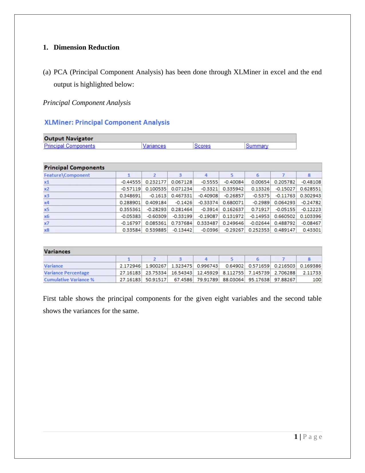
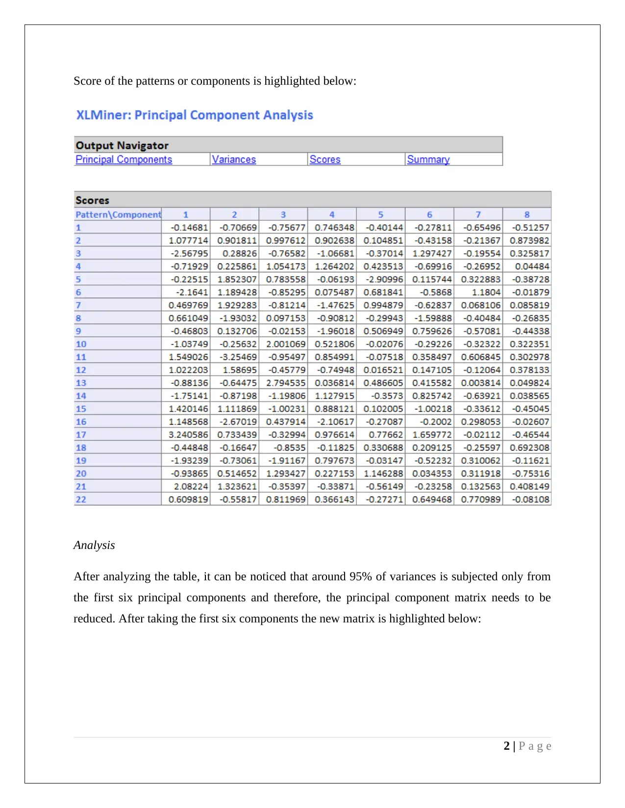
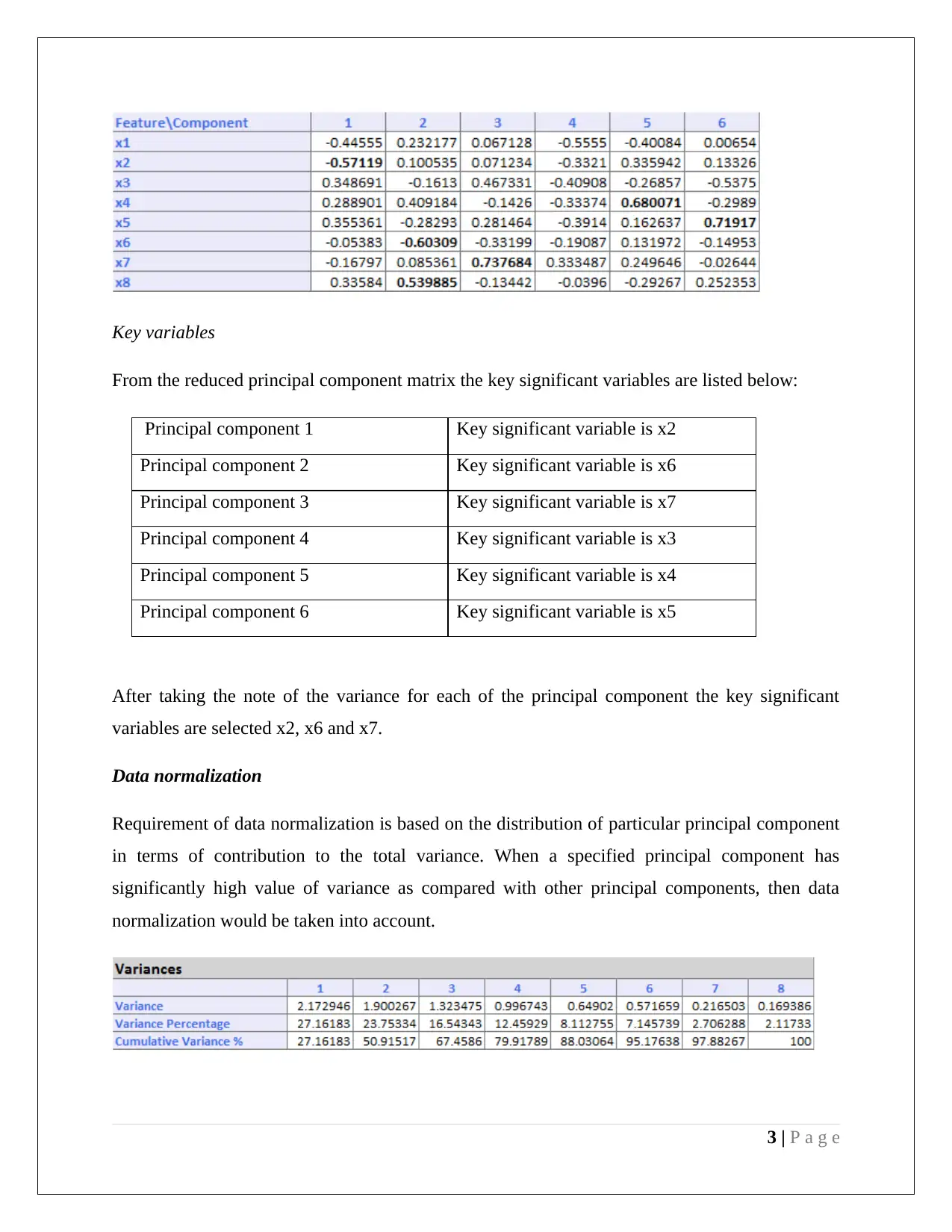
Homework Assignment
AI Summary
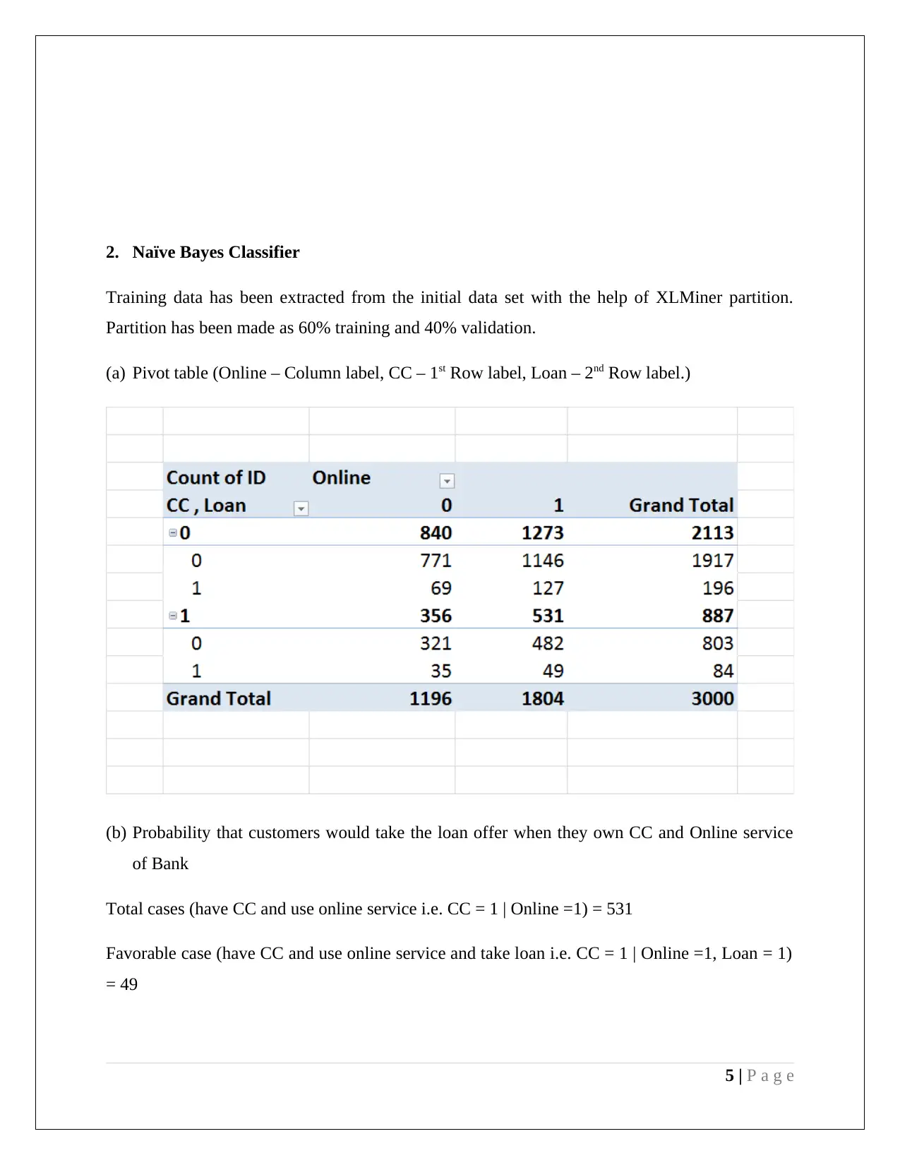
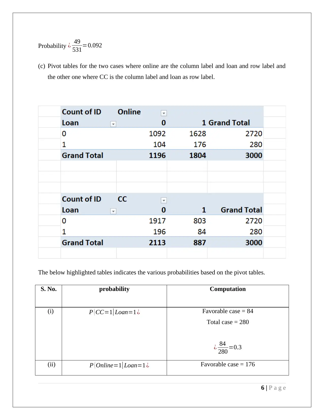
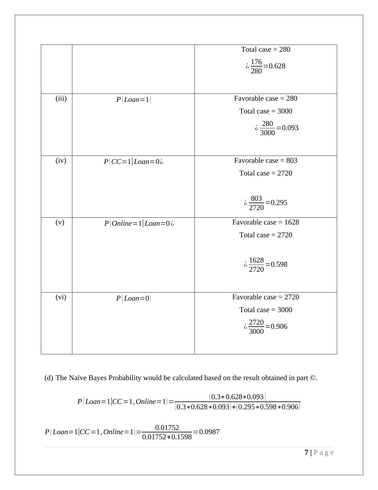
This document presents a comprehensive analysis of a data mining assignment focusing on two key techniques: Principal Component Analysis (PCA) and Naive Bayes classification. The PCA section details dimension reduction using XLMiner in Excel, identifying key variables from the reduced principal component matrix and discussing the need for data normalization based on variance. The advantages and disadvantages of employing PCA are also outlined. The Naive Bayes section involves training data extraction, partition, and pivot table creation to calculate the probability of customers taking a loan offer based on their credit card ownership and online service usage. The analysis culminates in the calculation of the Naive Bayes probability, demonstrating how customer profiles influence loan application likelihood.

1 out of 8
Related Documents


![Data Mining and Visualization Business Case Analysis Solution - [Date]](/_next/image/?url=https%3A%2F%2Fdesklib.com%2Fmedia%2Fimages%2Fa4c62573bfd04fc8a6d2208b43ae0344.jpg&w=256&q=75)
Your All-in-One AI-Powered Toolkit for Academic Success.
+13062052269
info@desklib.com
Available 24*7 on WhatsApp / Email
![[object Object]](/_next/static/media/star-bottom.7253800d.svg)
Copyright © 2020–2026 A2Z Services. All Rights Reserved. Developed and managed by ZUCOL.