Data Mining Assignment: XLMiner Output Analysis and Interpretation

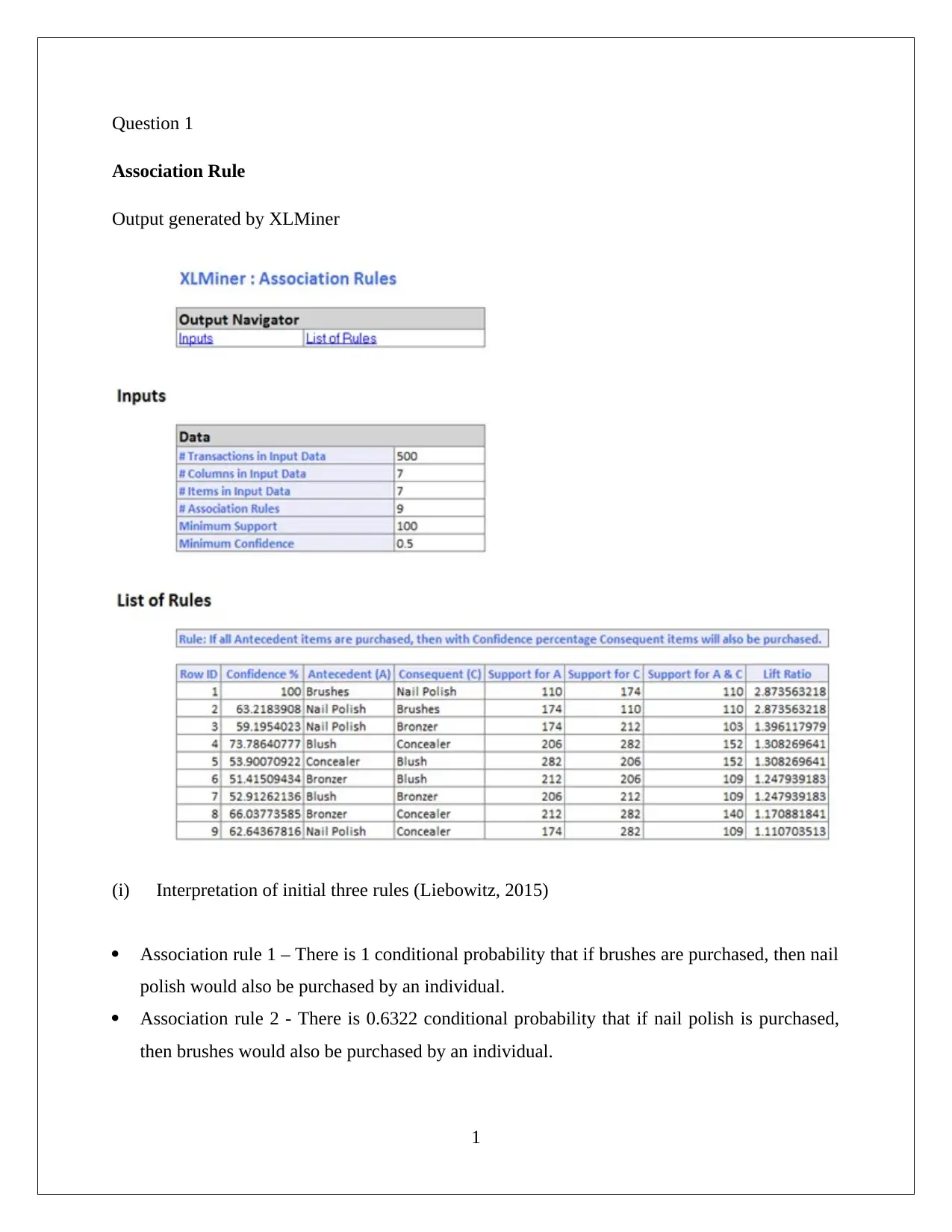
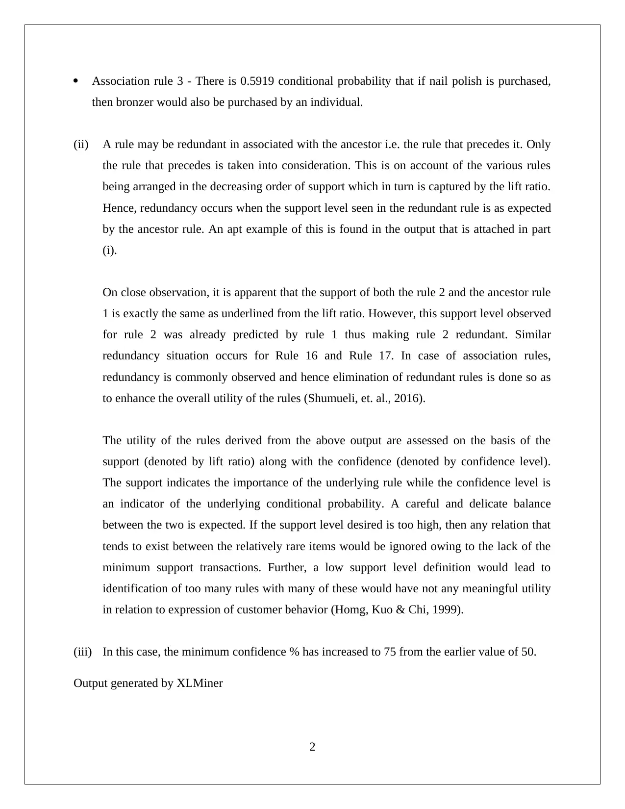
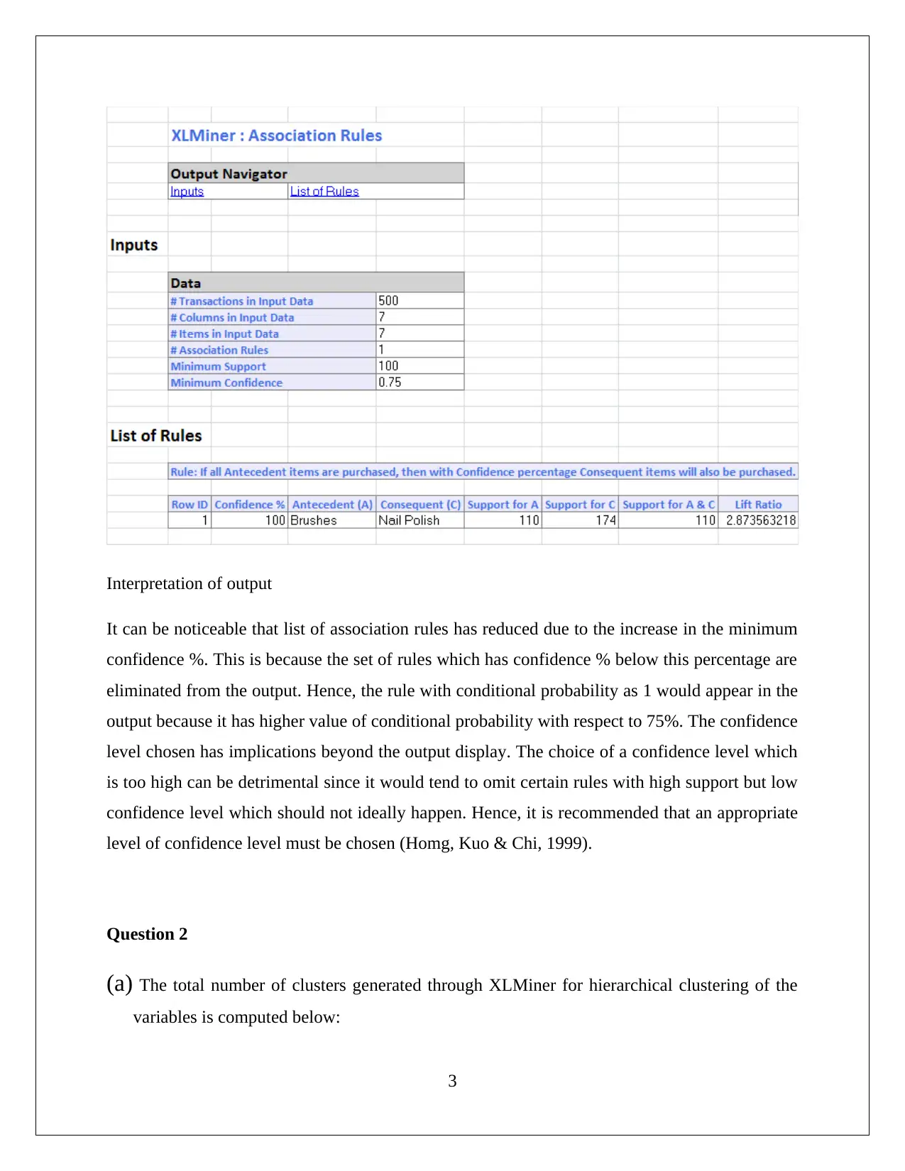
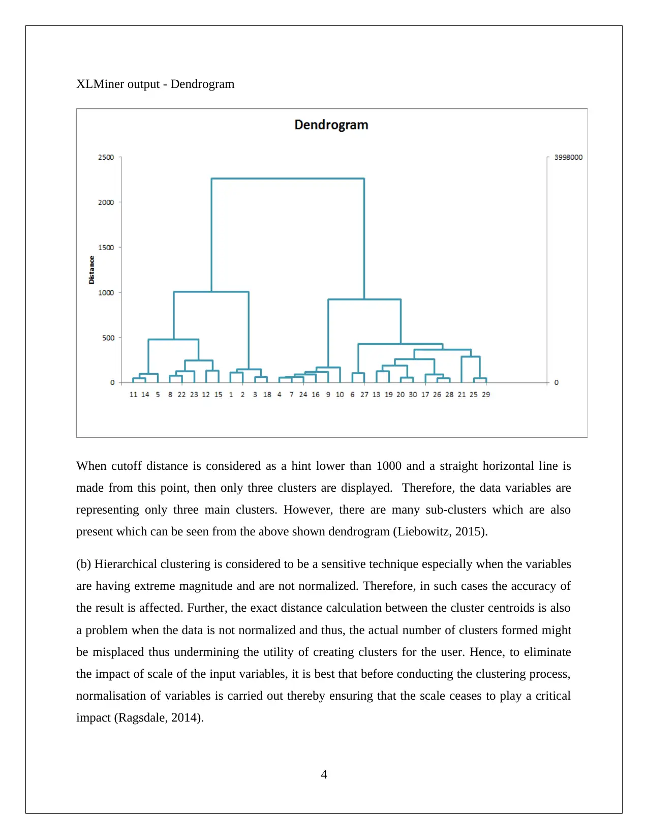
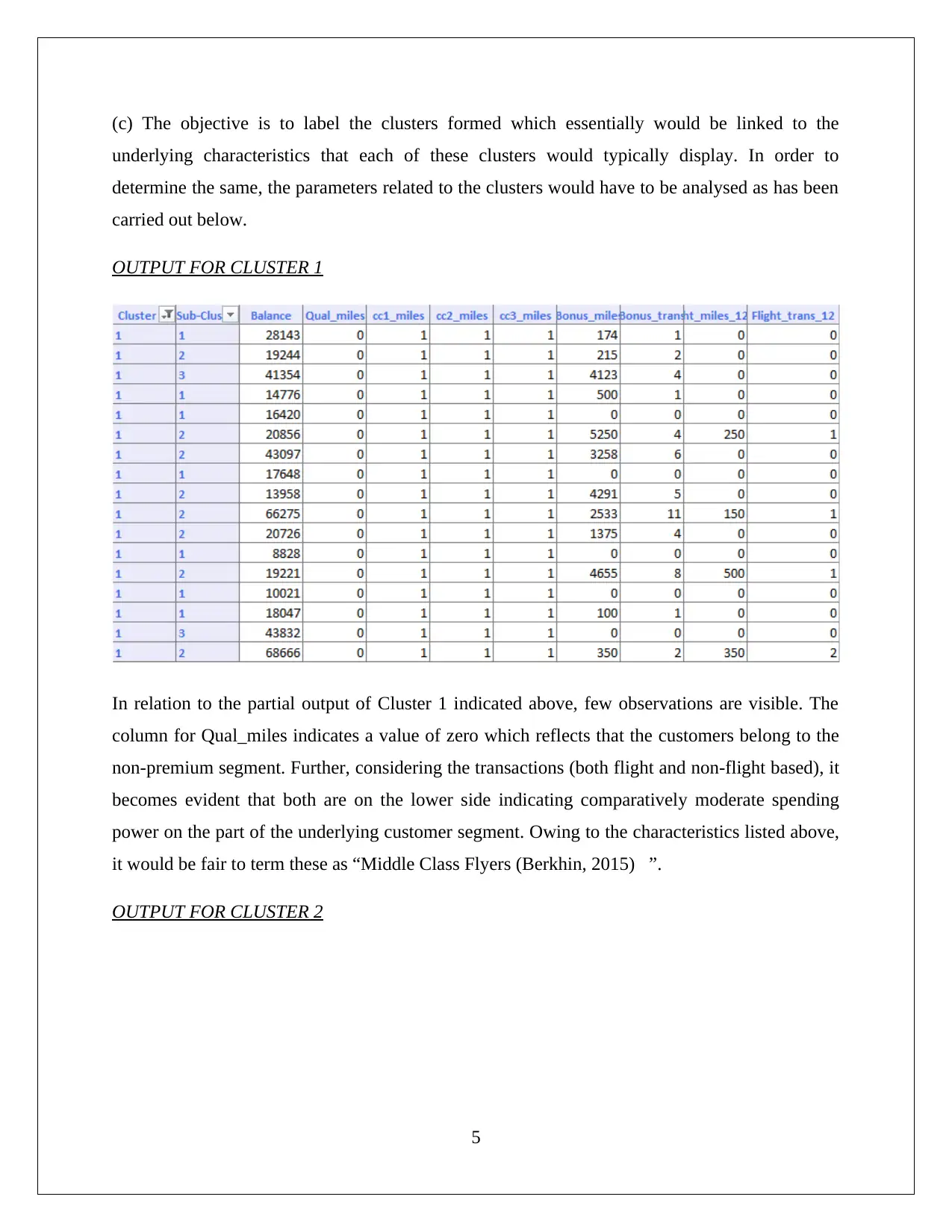
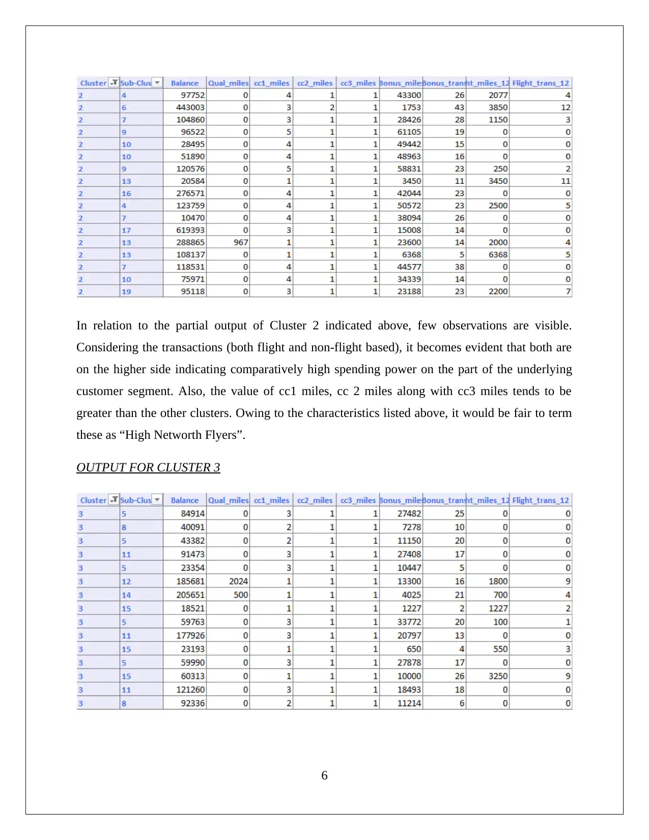
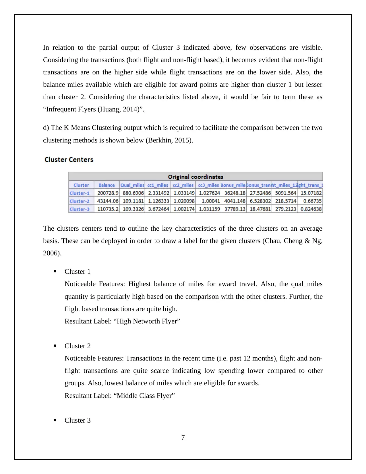
This data mining assignment delves into the analysis of association rules and clustering techniques using XLMiner. The solution begins by interpreting association rules, identifying redundancy based on support and lift ratios, and discussing the impact of confidence levels. It then explores hierarchical clustering, explaining the formation of clusters and the importance of data normalization. The assignment proceeds to label clusters based on their characteristics, differentiating between 'Middle Class Flyers,' 'High Networth Flyers,' and 'Infrequent Flyers.' Finally, it compares hierarchical and K-means clustering, providing cluster labels and suggesting targeted marketing offers for specific customer segments, such as encouraging increased flight transactions for 'Infrequent Flyers' and offering incentives for 'Middle Class Flyers'.

Data Mining
[Pick the date]
Student id

Question 1
Association Rule
Output generated by XLMiner
(i) Interpretation of initial three rules (Liebowitz, 2015)
 Association rule 1 – There is 1 conditional probability that if brushes are purchased, then nail
polish would also be purchased by an individual.
 Association rule 2 - There is 0.6322 conditional probability that if nail polish is purchased,
then brushes would also be purchased by an individual.
1

 Association rule 3 - There is 0.5919 conditional probability that if nail polish is purchased,
then bronzer would also be purchased by an individual.
(ii) A rule may be redundant in associated with the ancestor i.e. the rule that precedes it. Only
the rule that precedes is taken into consideration. This is on account of the various rules
being arranged in the decreasing order of support which in turn is captured by the lift ratio.
Hence, redundancy occurs when the support level seen in the redundant rule is as expected
by the ancestor rule. An apt example of this is found in the output that is attached in part
(i).
On close observation, it is apparent that the support of both the rule 2 and the ancestor rule
1 is exactly the same as underlined from the lift ratio. However, this support level observed
for rule 2 was already predicted by rule 1 thus making rule 2 redundant. Similar
redundancy situation occurs for Rule 16 and Rule 17. In case of association rules,
redundancy is commonly observed and hence elimination of redundant rules is done so as
to enhance the overall utility of the rules (Shumueli, et. al., 2016).
The utility of the rules derived from the above output are assessed on the basis of the
support (denoted by lift ratio) along with the confidence (denoted by confidence level).
The support indicates the importance of the underlying rule while the confidence level is
an indicator of the underlying conditional probability. A careful and delicate balance
between the two is expected. If the support level desired is too high, then any relation that
tends to exist between the relatively rare items would be ignored owing to the lack of the
minimum support transactions. Further, a low support level definition would lead to
identification of too many rules with many of these would have not any meaningful utility
in relation to expression of customer behavior (Homg, Kuo & Chi, 1999).
(iii) In this case, the minimum confidence % has increased to 75 from the earlier value of 50.
Output generated by XLMiner
2

Interpretation of output
It can be noticeable that list of association rules has reduced due to the increase in the minimum
confidence %. This is because the set of rules which has confidence % below this percentage are
eliminated from the output. Hence, the rule with conditional probability as 1 would appear in the
output because it has higher value of conditional probability with respect to 75%. The confidence
level chosen has implications beyond the output display. The choice of a confidence level which
is too high can be detrimental since it would tend to omit certain rules with high support but low
confidence level which should not ideally happen. Hence, it is recommended that an appropriate
level of confidence level must be chosen (Homg, Kuo & Chi, 1999).
Question 2
(a) The total number of clusters generated through XLMiner for hierarchical clustering of the
variables is computed below:
3

XLMiner output - Dendrogram
When cutoff distance is considered as a hint lower than 1000 and a straight horizontal line is
made from this point, then only three clusters are displayed. Therefore, the data variables are
representing only three main clusters. However, there are many sub-clusters which are also
present which can be seen from the above shown dendrogram (Liebowitz, 2015).
(b) Hierarchical clustering is considered to be a sensitive technique especially when the variables
are having extreme magnitude and are not normalized. Therefore, in such cases the accuracy of
the result is affected. Further, the exact distance calculation between the cluster centroids is also
a problem when the data is not normalized and thus, the actual number of clusters formed might
be misplaced thus undermining the utility of creating clusters for the user. Hence, to eliminate
the impact of scale of the input variables, it is best that before conducting the clustering process,
normalisation of variables is carried out thereby ensuring that the scale ceases to play a critical
impact (Ragsdale, 2014).
4

(c) The objective is to label the clusters formed which essentially would be linked to the
underlying characteristics that each of these clusters would typically display. In order to
determine the same, the parameters related to the clusters would have to be analysed as has been
carried out below.
OUTPUT FOR CLUSTER 1
In relation to the partial output of Cluster 1 indicated above, few observations are visible. The
column for Qual_miles indicates a value of zero which reflects that the customers belong to the
non-premium segment. Further, considering the transactions (both flight and non-flight based), it
becomes evident that both are on the lower side indicating comparatively moderate spending
power on the part of the underlying customer segment. Owing to the characteristics listed above,
it would be fair to term these as “Middle Class Flyers (Berkhin, 2015) ”.
OUTPUT FOR CLUSTER 2
5

In relation to the partial output of Cluster 2 indicated above, few observations are visible.
Considering the transactions (both flight and non-flight based), it becomes evident that both are
on the higher side indicating comparatively high spending power on the part of the underlying
customer segment. Also, the value of cc1 miles, cc 2 miles along with cc3 miles tends to be
greater than the other clusters. Owing to the characteristics listed above, it would be fair to term
these as “High Networth Flyers”.
OUTPUT FOR CLUSTER 3
6

In relation to the partial output of Cluster 3 indicated above, few observations are visible.
Considering the transactions (both flight and non-flight based), it becomes evident that non-flight
transactions are on the higher side while flight transactions are on the lower side. Also, the
balance miles available which are eligible for award points are higher than cluster 1 but lesser
than cluster 2. Considering the characteristics listed above, it would be fair to term these as
“Infrequent Flyers (Huang, 2014)”.
d) The K Means Clustering output which is required to facilitate the comparison between the two
clustering methods is shown below (Berkhin, 2015).
The clusters centers tend to outline the key characteristics of the three clusters on an average
basis. These can be deployed in order to draw a label for the given clusters (Chau, Cheng & Ng,
2006).
 Cluster 1
Noticeable Features: Highest balance of miles for award travel. Also, the qual_miles
quantity is particularly high based on the comparison with the other clusters. Further, the
flight based transactions are quite high.
Resultant Label: “High Networth Flyer”
 Cluster 2
Noticeable Features: Transactions in the recent time (i.e. past 12 months), flight and non-
flight transactions are quite scarce indicating low spending lower compared to other
groups. Also, lowest balance of miles which are eligible for awards.
Resultant Label: “Middle Class Flyer”
 Cluster 3
7

Noticeable Features: Transactions in the recent time (i.e. past 12 months), flight
transactions are quite scarce but non-flight based transactions are significantly higher.
Resultant Label: “Infrequent Flyer”
(e) One of the clusters that is to targeted is cluster 3 which is quite substantial. The relevant offer
would be one which can ensure that this segment engages in higher flight based transactions.
One way to ensure this is usage of available bonus points in flight to non-flight model in the ratio
of 80:20 (Chau, Cheng & Ng, 2006).
Also, cluster 2 is also a target potential. Incentive in the offer of higher reward points for miles
on transactions enabled through frequent flyer card is suggested to enhance business from this
segment (Ana, 2014).
8

Reference
Ana, A. (2014) Integration of Data Mining in Business Intelligence System (4th ed.). Sydney:
IGA Global
Berkhin, P. (2015). Survey of clustering Data Mining Techniques. Accrue software, Inc. 123-47.
https://www.cc.gatech.edu/~isbell/reading/papers/berkhin02survey.pdf
Chau, m., Cheng, R., Kao, B. & Ng, J. (2006). Uncertain Data Mining: An Example in clustering
Location Data. Retrieved from https://link.springer.com/chapter/10.1007%2F11731139_24
Hong, P.T., Kuo, S.C., & Chi, C.S. (1999). Mining Association Rue From Quantitative Data.
Intelligent Data Analysis. Vol (3), 363-376.
http://www.sciencedirect.com/science/article/pii/S1088467X99000281
Huang, Z. (2014). Clustering Large Data Sets with Mixed Numeric and Categorical Values.
CSIRO Mathematical and Information Sciences. 16(2), 45-78.
https://grid.cs.gsu.edu/~wkim/index_files/papers/kprototype.pdf
Liebowitz, J. (2015) Business Analytics: An Introduction (2nd ed.). New York: CRC Press.
Ragsdale, C. (2014) Spread sheet Modeling and Decision Analysis: A Practical Introduction to
Business Analytics (7th ed.). London: Cengage Learning.
Shumueli, G., Bruce, C.P., Yahav, I., Patel, R. N., Kenneth, C., & Lichtendahl, J. (2016) Data
Mining For Business Analytics: Concepts Techniques and Application (2nd ed.).London:
John Wiley & Sons.
9