Data Mining & Visualization: Business Intelligence Assignment Analysis
VerifiedAdded on 2020/04/01
|10
|985
|56
Homework Assignment
AI Summary
This document presents a comprehensive solution to a Data Mining and Visualization assignment, focusing on the application of Principal Component Analysis (PCA) and Naive Bayes methods for business intelligence. The solution begins by analyzing a utility dataset using PCA in XLMiner, interpreting the results to reduce the principal components and identify key variables like rate of return, sales, and nuclear percentage. The analysis includes data normalization considerations and a discussion of the advantages and disadvantages of the PCA method. The second part of the solution addresses data partitioning and the use of pivot tables to compute probabilities for customer loan acceptance based on online service usage and credit card ownership. The Naive Bayes probability is calculated, and a strategy for customer loan offers is suggested. The document references several key sources, providing a robust and well-supported analysis of the data mining concepts.

Data Mining and Visualization for Business Intelligence
Assignment - 2
[Pick the date]
Student Number and Name
Assignment - 2
[Pick the date]
Student Number and Name
Paraphrase This Document
Need a fresh take? Get an instant paraphrase of this document with our AI Paraphraser
Data Mining & Visualization
Question 1
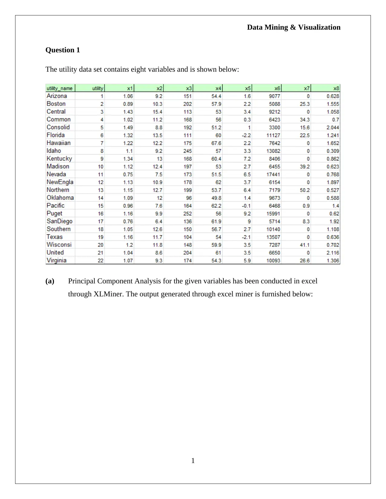
The utility data set contains eight variables and is shown below:
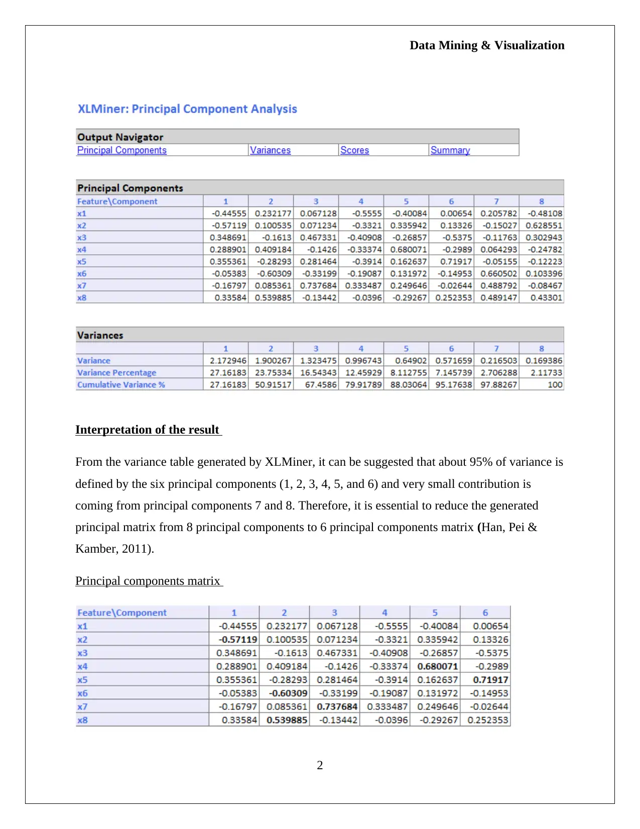
(a) Principal Component Analysis for the given variables has been conducted in excel
through XLMiner. The output generated through excel miner is furnished below:
1
Question 1
The utility data set contains eight variables and is shown below:
(a) Principal Component Analysis for the given variables has been conducted in excel
through XLMiner. The output generated through excel miner is furnished below:
1
Data Mining & Visualization
Interpretation of the result
From the variance table generated by XLMiner, it can be suggested that about 95% of variance is
defined by the six principal components (1, 2, 3, 4, 5, and 6) and very small contribution is
coming from principal components 7 and 8. Therefore, it is essential to reduce the generated
principal matrix from 8 principal components to 6 principal components matrix (Han, Pei &
Kamber, 2011).
Principal components matrix
2
⊘ This is a preview!⊘
Do you want full access?
Subscribe today to unlock all pages.

Trusted by 1+ million students worldwide
Data Mining & Visualization
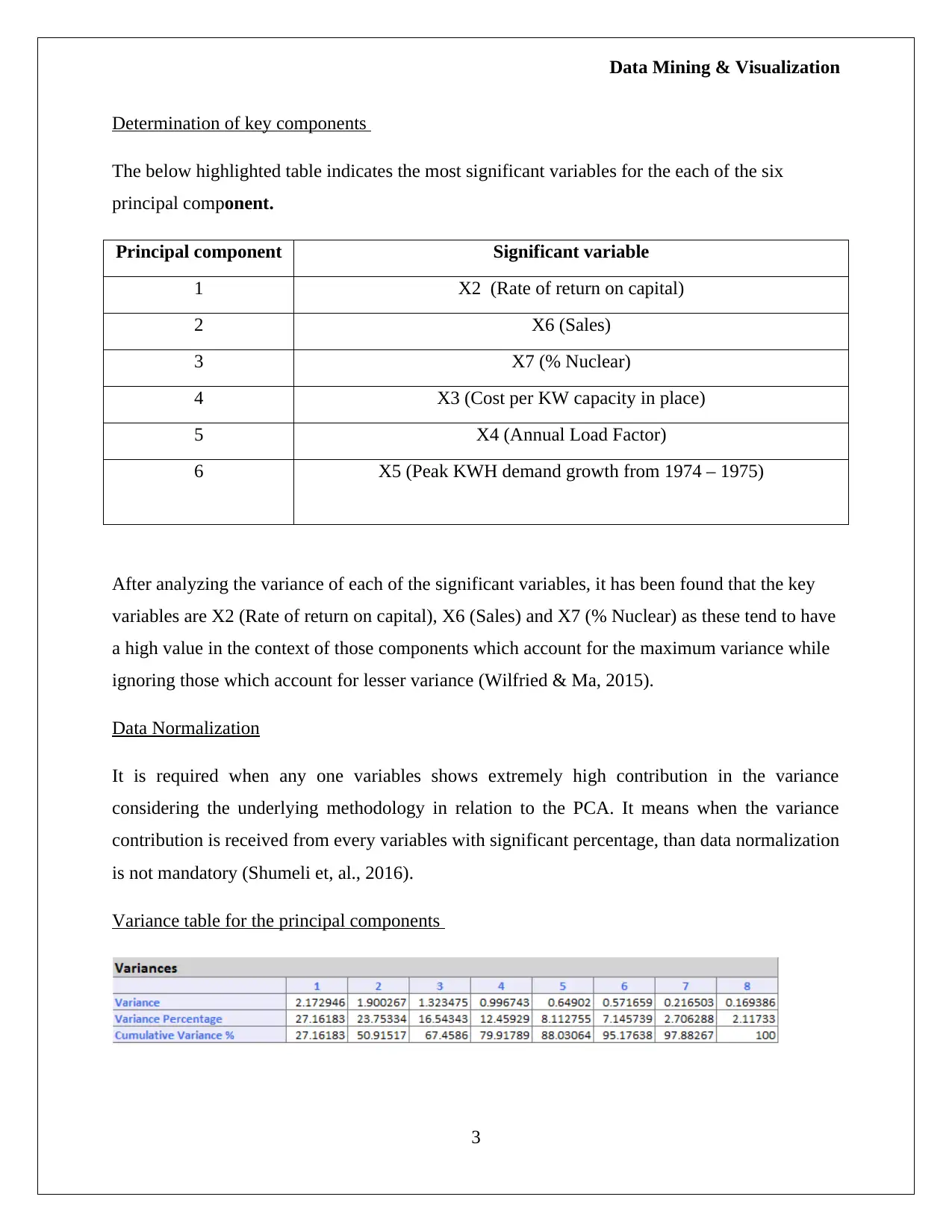
Determination of key components
The below highlighted table indicates the most significant variables for the each of the six
principal component.
Principal component Significant variable
1 X2 (Rate of return on capital)
2 X6 (Sales)
3 X7 (% Nuclear)
4 X3 (Cost per KW capacity in place)
5 X4 (Annual Load Factor)
6 X5 (Peak KWH demand growth from 1974 – 1975)
After analyzing the variance of each of the significant variables, it has been found that the key
variables are X2 (Rate of return on capital), X6 (Sales) and X7 (% Nuclear) as these tend to have
a high value in the context of those components which account for the maximum variance while
ignoring those which account for lesser variance (Wilfried & Ma, 2015).
Data Normalization
It is required when any one variables shows extremely high contribution in the variance
considering the underlying methodology in relation to the PCA. It means when the variance
contribution is received from every variables with significant percentage, than data normalization
is not mandatory (Shumeli et, al., 2016).
Variance table for the principal components
3
Paraphrase This Document
Need a fresh take? Get an instant paraphrase of this document with our AI Paraphraser
Data Mining & Visualization
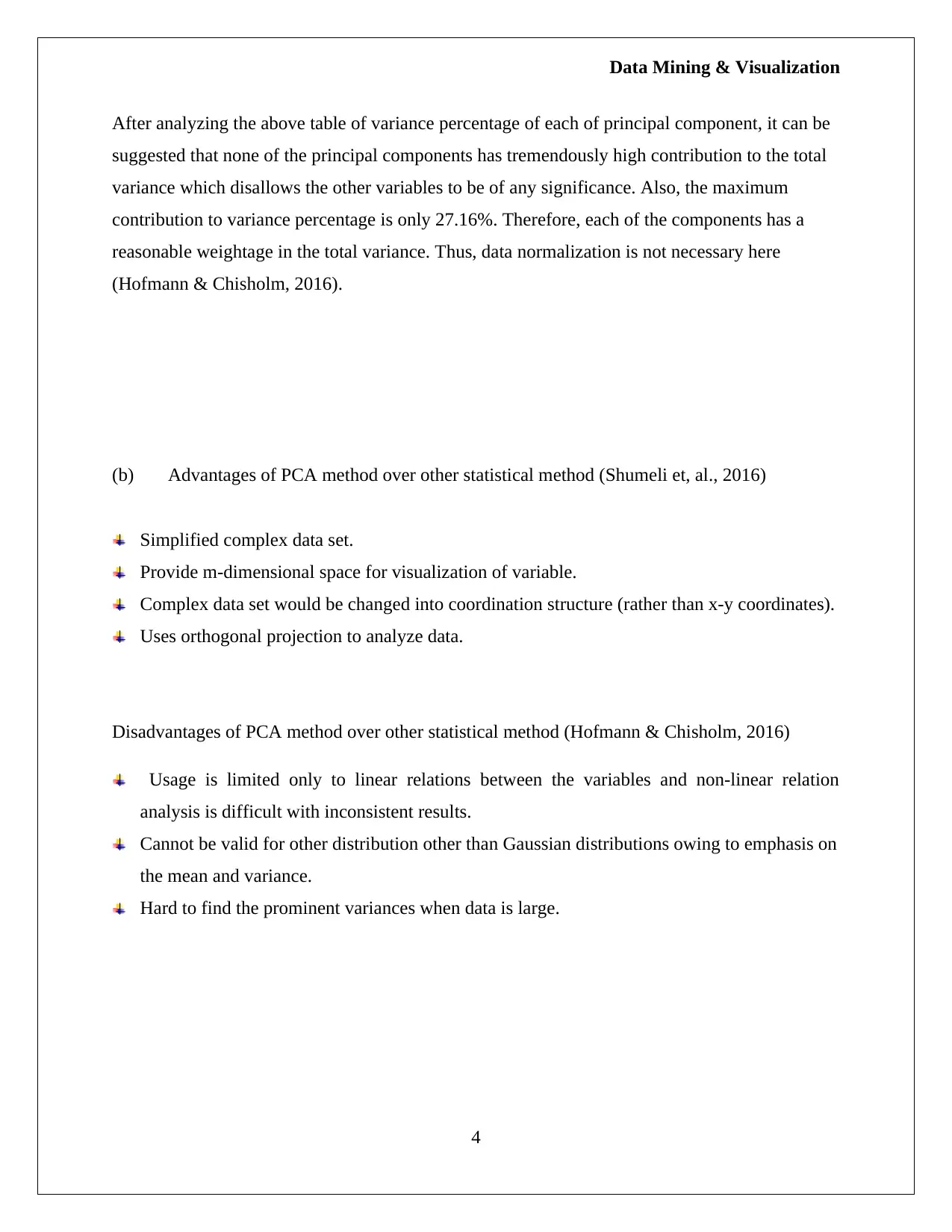
After analyzing the above table of variance percentage of each of principal component, it can be
suggested that none of the principal components has tremendously high contribution to the total
variance which disallows the other variables to be of any significance. Also, the maximum
contribution to variance percentage is only 27.16%. Therefore, each of the components has a
reasonable weightage in the total variance. Thus, data normalization is not necessary here
(Hofmann & Chisholm, 2016).
(b) Advantages of PCA method over other statistical method (Shumeli et, al., 2016)
Simplified complex data set.
Provide m-dimensional space for visualization of variable.
Complex data set would be changed into coordination structure (rather than x-y coordinates).
Uses orthogonal projection to analyze data.
Disadvantages of PCA method over other statistical method (Hofmann & Chisholm, 2016)
Usage is limited only to linear relations between the variables and non-linear relation
analysis is difficult with inconsistent results.
Cannot be valid for other distribution other than Gaussian distributions owing to emphasis on
the mean and variance.
Hard to find the prominent variances when data is large.
4
Data Mining & Visualization
Question 2
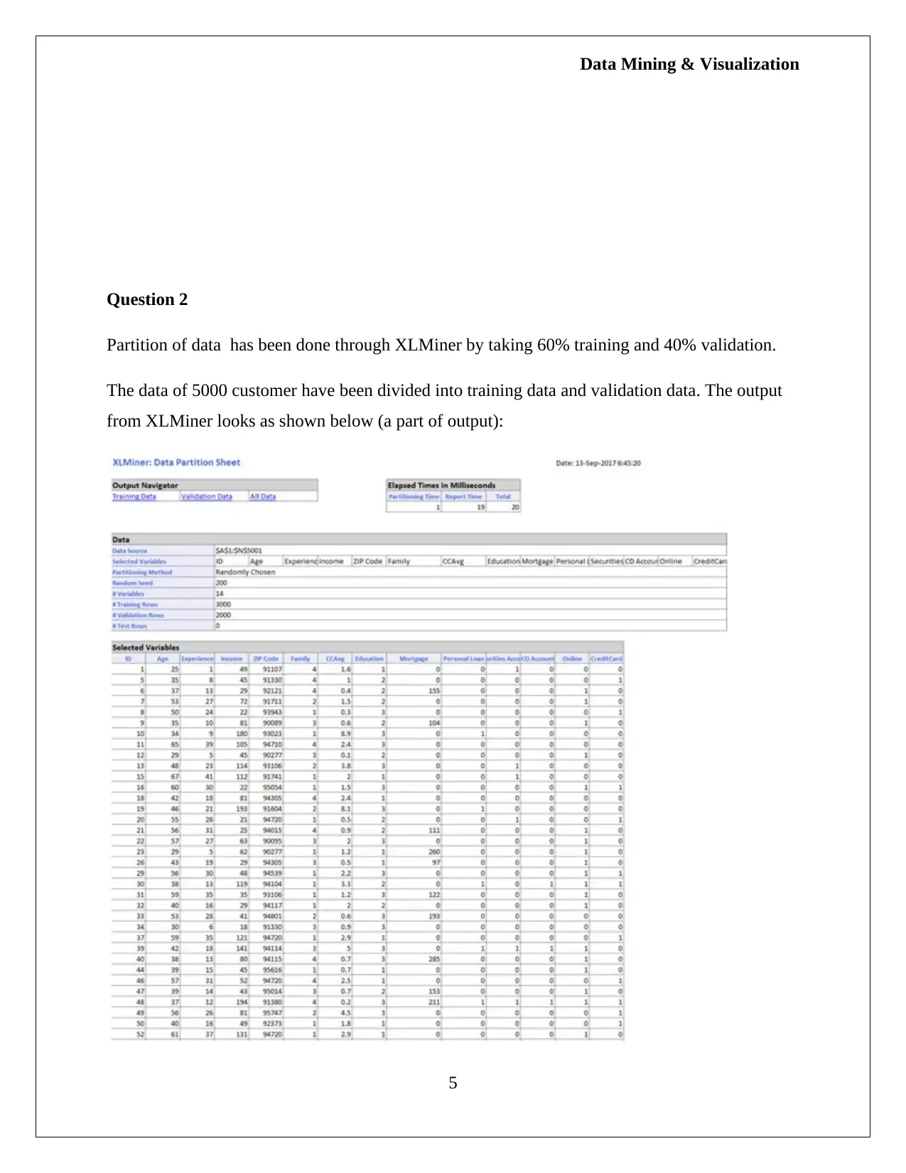
Partition of data has been done through XLMiner by taking 60% training and 40% validation.
The data of 5000 customer have been divided into training data and validation data. The output
from XLMiner looks as shown below (a part of output):
5
Question 2
Partition of data has been done through XLMiner by taking 60% training and 40% validation.
The data of 5000 customer have been divided into training data and validation data. The output
from XLMiner looks as shown below (a part of output):
5
⊘ This is a preview!⊘
Do you want full access?
Subscribe today to unlock all pages.

Trusted by 1+ million students worldwide
Data Mining & Visualization
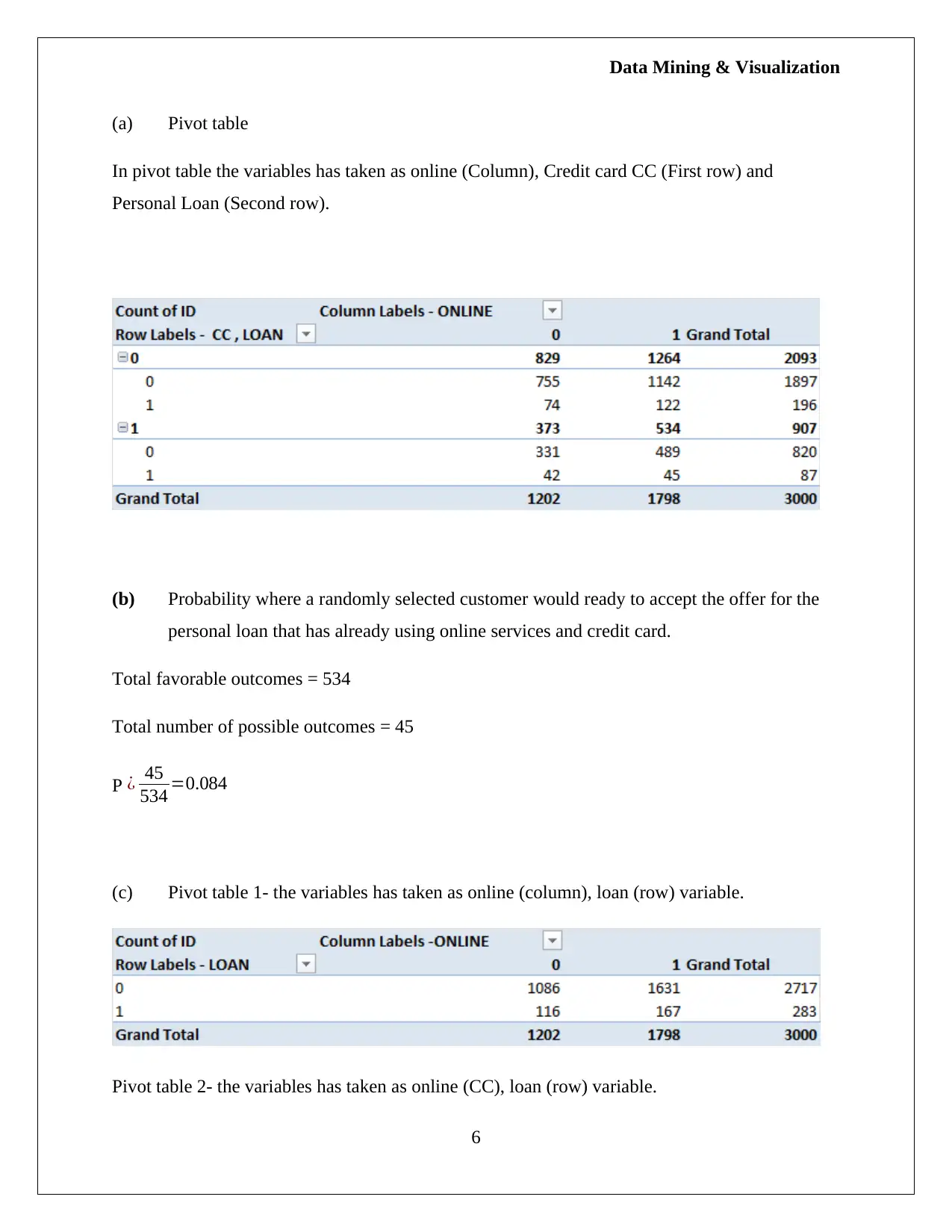
(a) Pivot table
In pivot table the variables has taken as online (Column), Credit card CC (First row) and
Personal Loan (Second row).
(b) Probability where a randomly selected customer would ready to accept the offer for the
personal loan that has already using online services and credit card.
Total favorable outcomes = 534
Total number of possible outcomes = 45
P ¿ 45
534 =0.084
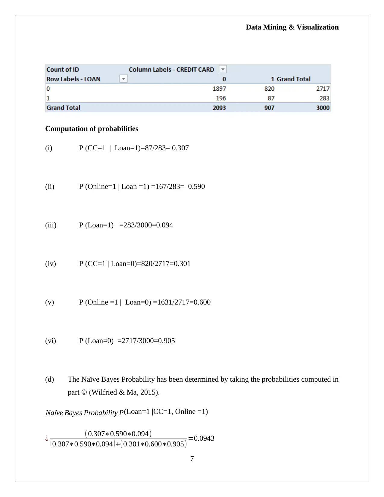
(c) Pivot table 1- the variables has taken as online (column), loan (row) variable.
Pivot table 2- the variables has taken as online (CC), loan (row) variable.
6
Paraphrase This Document
Need a fresh take? Get an instant paraphrase of this document with our AI Paraphraser
Data Mining & Visualization
Computation of probabilities
(i) P (CC=1 | Loan=1)=87/283= 0.307
(ii) P (Online=1 | Loan =1) =167/283= 0.590
(iii) P (Loan=1) =283/3000=0.094
(iv) P (CC=1 | Loan=0)=820/2717=0.301
(v) P (Online =1 | Loan=0) =1631/2717=0.600
(vi) P (Loan=0) =2717/3000=0.905
(d) The Naïve Bayes Probability has been determined by taking the probabilities computed in
part © (Wilfried & Ma, 2015).
Naïve Bayes Probability P(Loan=1 |CC=1, Online =1)
¿ (0.307∗0.590∗0.094)
( 0.307∗0.590∗0.094 ) +(0.301∗0.600∗0.905) =0.0943
7

Data Mining & Visualization
Therefore, value of Naïve Bayes Probability is 0.0943.
(e) The best possible strategy for the customer to get the loan is to have a credit card issued
from the same bank while not be a regular user of the online services that the bank offers.
This would help in higher probability of loan being offered by the bank.
8
⊘ This is a preview!⊘
Do you want full access?
Subscribe today to unlock all pages.

Trusted by 1+ million students worldwide
Data Mining & Visualization
References
G. Wilfried & Ma, R.S. (2015) Fundamentals of Business Intelligence (4th ed.). London: Springer
Publication.
Han, J., Pei, J. & Kamber, M. (2011) Data Mining Concept and Techniques (3rd ed.). New York:
Elsevier.
Hofmann, M. & Chisholm, A. (2016) Text Mining and Visualization: Case Studies Using Open-
source Tools. Sydney: CRC Press.
Shmueli, G. Bruce, C.P., Stephens, L.M. & Patel, R. N. (2016) Data Mining for Business
Analytics Concepts, Techniques and Applications with JMP Pro. Sydney: John Wiley &
Sons.
9
1 out of 10
Related Documents
Your All-in-One AI-Powered Toolkit for Academic Success.
+13062052269
info@desklib.com
Available 24*7 on WhatsApp / Email
![[object Object]](/_next/static/media/star-bottom.7253800d.svg)
Unlock your academic potential
Copyright © 2020–2026 A2Z Services. All Rights Reserved. Developed and managed by ZUCOL.


