Business Analytics (ISYS3374) Assignment 3: Data Analysis and Insights

This assignment solution for ISYS3374, a Business Analytics course at RMIT University, addresses various data analysis and modeling techniques. It begins by defining overfitting and suggesting methods to avoid it, followed by an exploration of predictive analytics in retail, including forecasting and customer behavior analysis. The solution then discusses missing not at random (MNAR) values, suggesting multiple-regression analysis for handling them, and explains the development of a logistic regression model using dummy variables. Section B provides detailed regression analysis outputs, model evaluations, and recommendations for improvement. It includes analysis of repair time, profit calculations, and missing data handling using stratified sampling, pivot tables, and charts. Finally, the solution presents a multiple regression model to predict diabetes risk, incorporating age, weight, and gender, along with interpretation and application of the formula to predict individual risk.

School name: RMIT University
1-
Course/Unit code Assignment
number
Assignment
due date
Group/Session name (if applicable)
ISYS3374 Assignment 3 31 May 2020
Course/Unit name Program title
Business Analytics (2010) Master Business of Information Technology
Lecturer/Teacher’s name Tutor / Marker’s name (if applicable)
Dr Babak Abbasi Dr Joerin Motavallian
This statement should be completed and signed by the student(s) participating in preparation of the
assignment.
Declaration and statement of authorship:
1. I/we hold a copy of this assignment, which can be produced if the original is lost/damaged.
2. This assignment is my/our original work and no part of it has been copied from any other student’s work or from any other
source except where due acknowledgment is made.
3. No part of this assignment has been written for me/us by any other person except where such collaboration has been authorised
by the lecturer/teacher concerned and is clearly acknowledged in the assignment.
4. I/we have not previously submitted or currently submitting this work for any other course/unit.
5. This work may be reproduced and/or communicated for the purpose of detecting plagiarism.
6. I/we give permission for a copy of my/our marked work to be retained by the School for review by external examiners.
7. I/we understand that plagiarism is the presentation of the work, idea or creation of another person as though it is your own. It is
a form of cheating and is a very serious academic offence that may lead to expulsion from the University. Plagiarised material
can be drawn from, and presented in, written, graphic and visual form, including electronic data, and oral presentations.
Plagiarism occurs when the origin of the material used is not appropriately cited.
8. Enabling plagiarism is the act of assisting or allowing another person to plagiarise or to copy your work.
Family name Given name Student number Student signature Date
LY TRONG TIEN S3790425 31 May 2020
Further information relating to the penalties for plagiarism, which range from a notation on your student file to expulsion from the
University, is contained in Regulation 6.1.1 ‘Student Discipline’ www.rmit.edu.au/browse;ID=11jgnnjgg70y and Academic Policy:
‘Plagiarism’ www.rmit.edu.au/browse;ID=sg4yfqzod48g1.
Assessor’s comments Grade School date stamp
(Office use only)

SECTION A:
Question 1:
Overfitting is when a model is too closely or exactly corresponding to a particular sample dataset
which may cause that model not able to match with other sets of data, and therefore would provide
some inaccurate prediction. However, this is easy to avoid by some following techniques:
- Using just independent variables that have close and meaningful relationship with dependent
variable to lessen the risk of
- Using more complex models like linear regression models or quadratic models to test if the
model can generate accuracy value by evaluating its performance on a different set of data
and base on that can approximate the typical hidden data that could cause overfitting to the
model.
- Putting more data inside the sample dataset to increase the accuracy of testing.
Question 2:
Predictive analytics has been deployed to use in many industries, especially in retailing industry,
where it is considered as the most useful tool help forecasting the stocks and improving the
customer experience. Retailing businesses can have a better plan of stocking to avoid the over-stock
or out-of-stock problem. For instance, in the peak season like Christmas or Black Friday when the
demands of shopping increase, predictive analytics could use historical data to predict the amount of
goods could be sold to avoid out-of-stock in stores. Predictive analytics also provides a better insight
of customer behavior when analyzing the shopping preferences or the buying history in order to
predict new opportunities to engage with their customers, and when it comes to a new marketing or
sale campaign predictive analytics could help to build-up a better personalized shopping experience.
Question 3:
Missing not at random values is when that missing value has relationship with the attribute. To deal
with MNAR, there are many methods to do, but the most popular is to use multiple-regression
analysis to estimate a missing value. By using this technique to figure out the missing SUS scores.
Regression substitution could help to predict the missing value from the other values of the same
category. Example of not missing at random values is when doing an income survey, the people who
have higher income tend to hide their true income or don’t want to provide the answer cause
missing not at random in the final report.
Question 4:
To develop the logistic regression model, the variable X1 can be replaced by two dummy variables, in
which each would correspond to one of the levels of the X1 and have binary values of one and zero.
For instance, X1A and X1B can be used for X1. When X1A value is one and X1B is zero the category would
be low; or when X1A value is zero and X1B is one the category would be average; and when both have
the value of zero the category would be high. And the same rule is applied for X2 with three dummy
variables. Based on that, logistic regression model could be developed with five coefficients (two for
X1 and three for X2).
2

SECTION B:
Question 5:
Question 5 - Part a:
SUMMARY OUTPUT
Regression Statistics
Multiple R
0.06074
5
R Square 0.00369
Adjusted R Square -0.00436
Standard Error
295.826
7
Observations 500
ANOVA
df SS MS F
Significance
F
Regression 4 160435.8
40108.9
4
0.45831
7 0.766334
Residual 495
4331916
4
87513.4
6
Total 499
4347960
0
Coefficie
nts
Standard
Error t Stat P-value
Lower
95%
Upper
95%
Lower
95.0%
Upper
95.0%
Intercept 1164.20 48.642 23.93 1.12E-84 1068.6 1259.77 1068.63 1259.77
Age (blanks means
we do not know their
age) 0.84 0.7672 1.092 0.275 -0.6693 2.345 -0.669 2.345
Gender (Male is 1) -7.65 26.511 -0.288 0.772 -59.740 44.436 -59.74 44.436
Family size -6.04 7.7080 -0.783 0.433 -21.186 9.102 -21.186 9.102
Membership (with
membership is 1) -1.37 26.510 -0.051 0.958 -53.458 50.715 -53.458 50.715
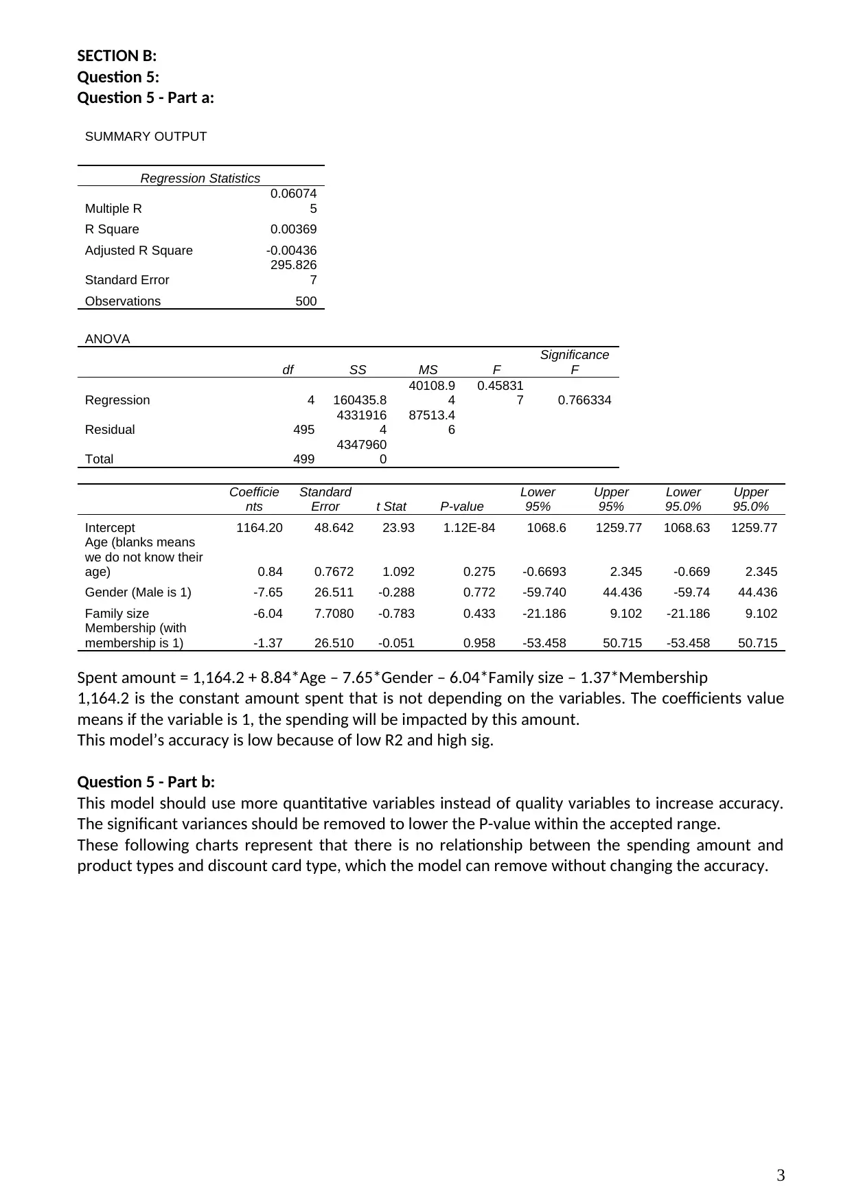
Spent amount = 1,164.2 + 8.84*Age – 7.65*Gender – 6.04*Family size – 1.37*Membership
1,164.2 is the constant amount spent that is not depending on the variables. The coefficients value
means if the variable is 1, the spending will be impacted by this amount.
This model’s accuracy is low because of low R2 and high sig.
Question 5 - Part b:
This model should use more quantitative variables instead of quality variables to increase accuracy.
The significant variances should be removed to lower the P-value within the accepted range.
These following charts represent that there is no relationship between the spending amount and
product types and discount card type, which the model can remove without changing the accuracy.
3

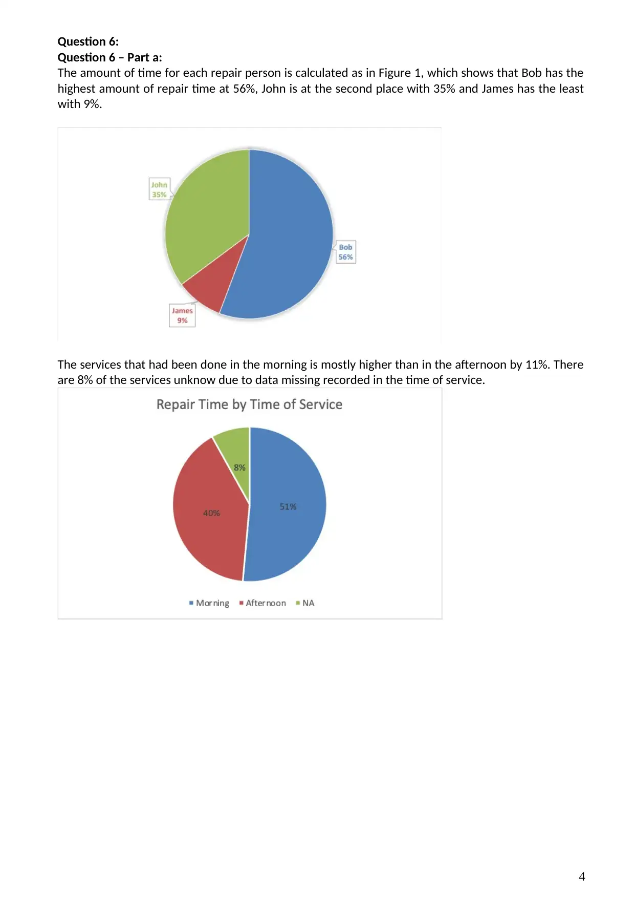
Question 6:
Question 6 – Part a:
The amount of time for each repair person is calculated as in Figure 1, which shows that Bob has the
highest amount of repair time at 56%, John is at the second place with 35% and James has the least
with 9%.
The services that had been done in the morning is mostly higher than in the afternoon by 11%. There
are 8% of the services unknow due to data missing recorded in the time of service.
4

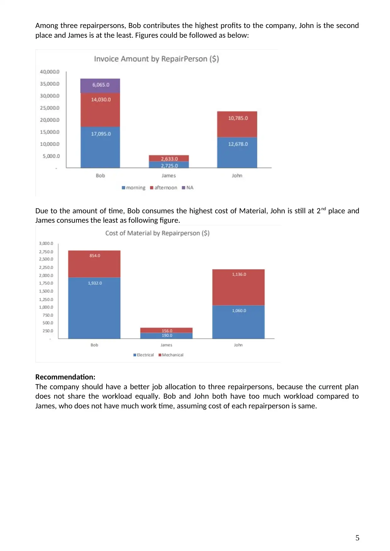
Among three repairpersons, Bob contributes the highest profits to the company, John is the second
place and James is at the least. Figures could be followed as below:
Due to the amount of time, Bob consumes the highest cost of Material, John is still at 2nd place and
James consumes the least as following figure.
Recommendation:
The company should have a better job allocation to three repairpersons, because the current plan
does not share the workload equally. Bob and John both have too much workload compared to
James, who does not have much work time, assuming cost of each repairperson is same.
5

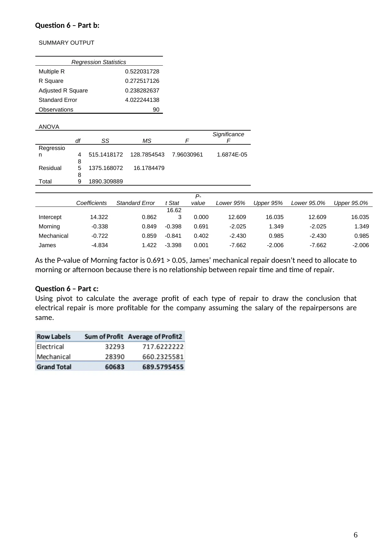
Question 6 – Part b:
SUMMARY OUTPUT
Regression Statistics
Multiple R 0.522031728
R Square 0.272517126
Adjusted R Square 0.238282637
Standard Error 4.022244138
Observations 90
ANOVA
df SS MS F
Significance
F
Regressio
n 4 515.1418172 128.7854543 7.96030961 1.6874E-05
Residual
8
5 1375.168072 16.1784479
Total
8
9 1890.309889
Coefficients Standard Error t Stat
P-
value Lower 95% Upper 95% Lower 95.0% Upper 95.0%
Intercept 14.322 0.862
16.62
3 0.000 12.609 16.035 12.609 16.035
Morning -0.338 0.849 -0.398 0.691 -2.025 1.349 -2.025 1.349
Mechanical -0.722 0.859 -0.841 0.402 -2.430 0.985 -2.430 0.985
James -4.834 1.422 -3.398 0.001 -7.662 -2.006 -7.662 -2.006
As the P-value of Morning factor is 0.691 > 0.05, James’ mechanical repair doesn’t need to allocate to
morning or afternoon because there is no relationship between repair time and time of repair.
Question 6 – Part c:
Using pivot to calculate the average profit of each type of repair to draw the conclusion that
electrical repair is more profitable for the company assuming the salary of the repairpersons are
same.
6

Question 7:
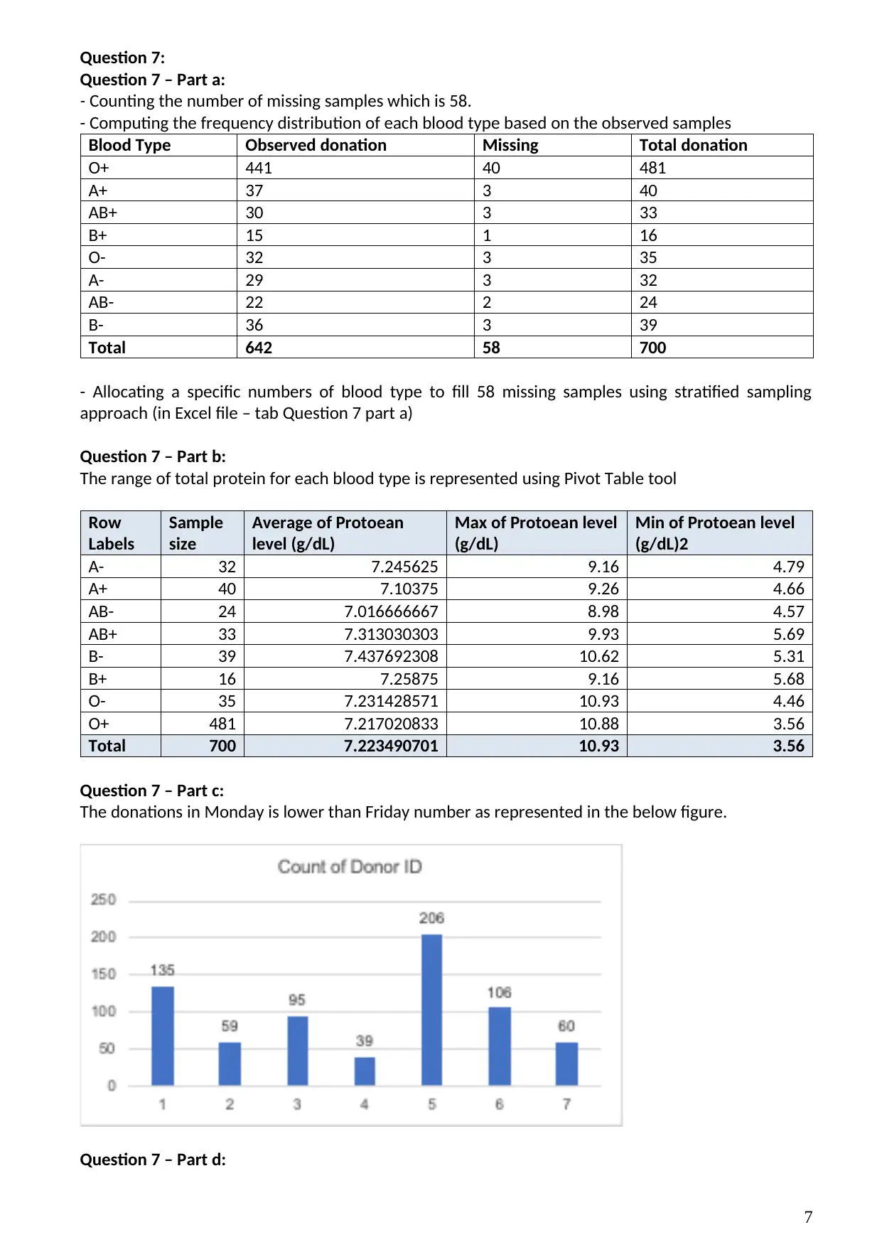
Question 7 – Part a:
- Counting the number of missing samples which is 58.
- Computing the frequency distribution of each blood type based on the observed samples
Blood Type Observed donation Missing Total donation
O+ 441 40 481
A+ 37 3 40
AB+ 30 3 33
B+ 15 1 16
O- 32 3 35
A- 29 3 32
AB- 22 2 24
B- 36 3 39
Total 642 58 700
- Allocating a specific numbers of blood type to fill 58 missing samples using stratified sampling
approach (in Excel file – tab Question 7 part a)
Question 7 – Part b:
The range of total protein for each blood type is represented using Pivot Table tool
Row
Labels
Sample
size
Average of Protoean
level (g/dL)
Max of Protoean level
(g/dL)
Min of Protoean level
(g/dL)2
A- 32 7.245625 9.16 4.79
A+ 40 7.10375 9.26 4.66
AB- 24 7.016666667 8.98 4.57
AB+ 33 7.313030303 9.93 5.69
B- 39 7.437692308 10.62 5.31
B+ 16 7.25875 9.16 5.68
O- 35 7.231428571 10.93 4.46
O+ 481 7.217020833 10.88 3.56
Total 700 7.223490701 10.93 3.56
Question 7 – Part c:
The donations in Monday is lower than Friday number as represented in the below figure.
Question 7 – Part d:
7

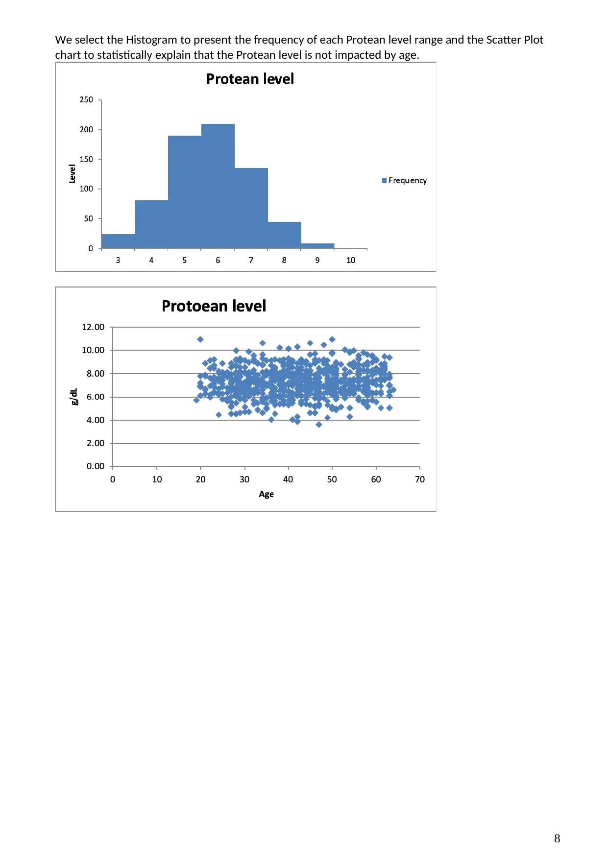
We select the Histogram to present the frequency of each Protean level range and the Scatter Plot
chart to statistically explain that the Protean level is not impacted by age.
8

Question 8:
Question 8 – Part a:
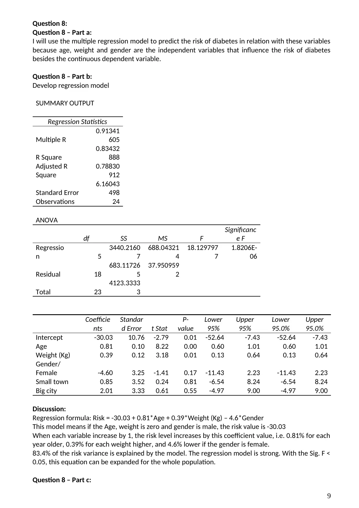
I will use the multiple regression model to predict the risk of diabetes in relation with these variables
because age, weight and gender are the independent variables that influence the risk of diabetes
besides the continuous dependent variable.
Question 8 – Part b:
Develop regression model
SUMMARY OUTPUT
Regression Statistics
Multiple R
0.91341
605
R Square
0.83432
888
Adjusted R
Square
0.78830
912
Standard Error
6.16043
498
Observations 24
ANOVA
df SS MS F
Significanc
e F
Regressio
n 5
3440.2160
7
688.04321
4
18.129797
7
1.8206E-
06
Residual 18
683.11726
5
37.950959
2
Total 23
4123.3333
3
Coefficie
nts
Standar
d Error t Stat
P-
value
Lower
95%
Upper
95%
Lower
95.0%
Upper
95.0%
Intercept -30.03 10.76 -2.79 0.01 -52.64 -7.43 -52.64 -7.43
Age 0.81 0.10 8.22 0.00 0.60 1.01 0.60 1.01
Weight (Kg) 0.39 0.12 3.18 0.01 0.13 0.64 0.13 0.64
Gender/
Female -4.60 3.25 -1.41 0.17 -11.43 2.23 -11.43 2.23
Small town 0.85 3.52 0.24 0.81 -6.54 8.24 -6.54 8.24
Big city 2.01 3.33 0.61 0.55 -4.97 9.00 -4.97 9.00
Discussion:
Regression formula: Risk = -30.03 + 0.81*Age + 0.39*Weight (Kg) – 4.6*Gender
This model means if the Age, weight is zero and gender is male, the risk value is -30.03
When each variable increase by 1, the risk level increases by this coefficient value, i.e. 0.81% for each
year older, 0.39% for each weight higher, and 4.6% lower if the gender is female.
83.4% of the risk variance is explained by the model. The regression model is strong. With the Sig. F <
0.05, this equation can be expanded for the whole population.
Question 8 – Part c:
9

Applying the formula, the risk percentage is as below:
-30.03 + 0.81*(52 + 4) + 0.39*80 – 4.6 = 41.93%
There is 41.93% that a 52-year-old woman with 80 kg weight will get diabetes in the next 4 years.
10

Question 9:
Question 9 – Part a:
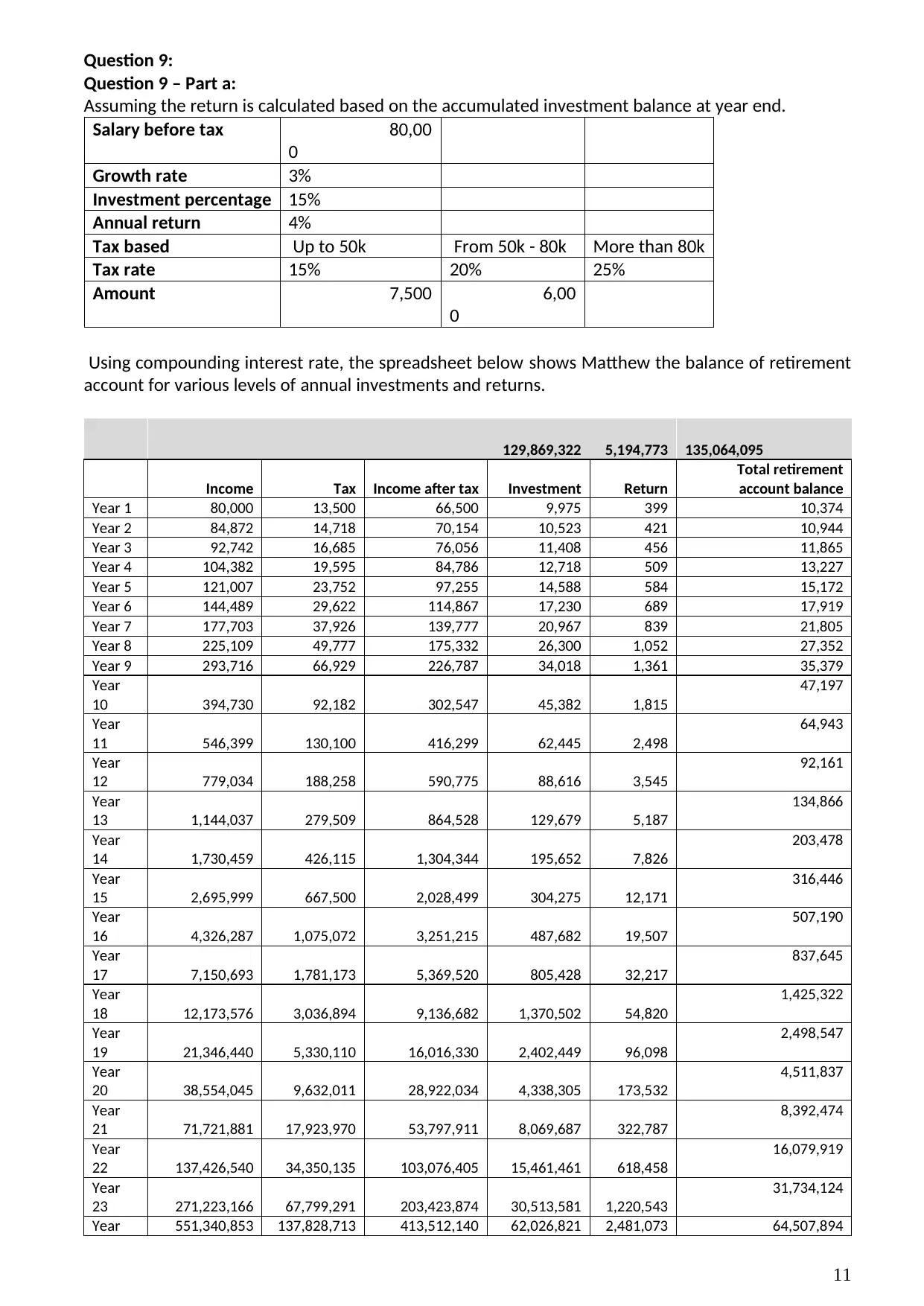
Assuming the return is calculated based on the accumulated investment balance at year end.
Salary before tax 80,00
0
Growth rate 3%
Investment percentage 15%
Annual return 4%
Tax based Up to 50k From 50k - 80k More than 80k
Tax rate 15% 20% 25%
Amount 7,500 6,00
0
Using compounding interest rate, the spreadsheet below shows Matthew the balance of retirement
account for various levels of annual investments and returns.
129,869,322 5,194,773 135,064,095
Income Tax Income after tax Investment Return
Total retirement
account balance
Year 1 80,000 13,500 66,500 9,975 399 10,374
Year 2 84,872 14,718 70,154 10,523 421 10,944
Year 3 92,742 16,685 76,056 11,408 456 11,865
Year 4 104,382 19,595 84,786 12,718 509 13,227
Year 5 121,007 23,752 97,255 14,588 584 15,172
Year 6 144,489 29,622 114,867 17,230 689 17,919
Year 7 177,703 37,926 139,777 20,967 839 21,805
Year 8 225,109 49,777 175,332 26,300 1,052 27,352
Year 9 293,716 66,929 226,787 34,018 1,361 35,379
Year
10 394,730 92,182 302,547 45,382 1,815
47,197
Year
11 546,399 130,100 416,299 62,445 2,498
64,943
Year
12 779,034 188,258 590,775 88,616 3,545
92,161
Year
13 1,144,037 279,509 864,528 129,679 5,187
134,866
Year
14 1,730,459 426,115 1,304,344 195,652 7,826
203,478
Year
15 2,695,999 667,500 2,028,499 304,275 12,171
316,446
Year
16 4,326,287 1,075,072 3,251,215 487,682 19,507
507,190
Year
17 7,150,693 1,781,173 5,369,520 805,428 32,217
837,645
Year
18 12,173,576 3,036,894 9,136,682 1,370,502 54,820
1,425,322
Year
19 21,346,440 5,330,110 16,016,330 2,402,449 96,098
2,498,547
Year
20 38,554,045 9,632,011 28,922,034 4,338,305 173,532
4,511,837
Year
21 71,721,881 17,923,970 53,797,911 8,069,687 322,787
8,392,474
Year
22 137,426,540 34,350,135 103,076,405 15,461,461 618,458
16,079,919
Year
23 271,223,166 67,799,291 203,423,874 30,513,581 1,220,543
31,734,124
Year 551,340,853 137,828,713 413,512,140 62,026,821 2,481,073 64,507,894
11

24
Year
25 1,154,385,310 288,589,827 865,795,482 129,869,322 5,194,773
35,064,095
12

Question 9 – Part b:
If the annual return rate is uncertain and it is between 5% to 9% in any given year, the expected
value (average) of Matthew balance after 25 years should be:
Sample size: 250
Expected retirement account balance: 130,580,456
Average interest balance: 711,134
13

Question 10:
Question 10 – Part a:
Assuming the discount will be applied for each material with order more than 10,000kg. Because
10,000kg of material A and material B is bought at discount price of $900 and $1,260kg, respectively,
the discount can only be made purchasing one of them. So the price before discount per kilo gram of
A and B respectively at $0.1 and $0.14 and price after discount is $0.09 and $0.126.
Because budget for raw martial is at $2,000 so either A or B would get the discount price, explained
by the equation:
10,000 kg A * $0.09 + 10,000 kg B *0.126 = $900 + $1,260 = $2,160  this is over budget.
So the company can only buy and get discount price for Martial A or Martial B as following equation:
Martial A*$0.09 + Martial B*$0.14 <= $2,000 (Martial A >=10,000 kg)
Or
Martial A*$1 + Martial B*$0.126 <= $2,000 (Martial B>=10,000 kg)
In which, for which martial that the company needs to produce Fertilizer 1 and 2 must follow the
rule:
Martial A amount >= 50% Fertilizer 1
Martial B amount >= 70% Fertilizer 2
To maximize profit, the company can use 3 equation below to estimate the amount of each Fertilizer
should produce:
- (50% Fertilizer 1 * $0.09) + (70% Fertilizer 2 * $0.14) <=$2,000
with the condition that Fertilizer 1 >= 20,000 kg
- (50% Fertilizer 1 * $1) + (70% Fertilizer 2 * $0.126) <= $2,000
With the condition that Fertilizer 2 >= 14,285.71 kg
- (50% Fertilizer 1 * $1) + (70% Fertilizer 2 * $0.14) <= $2,000
And the recommended number of unit (kg) that the company should use satisfies the equation:
Max = $60*Fertilizer 1 + $48*Fertilizer 2
Subject to:
- (50% Fertilizer 1 * $0.09) + (70% Fertilizer 2 * $0.14) <=$2,000; Fertilizer 1 >= 20,000 kg
- (50% Fertilizer 1 * $1) + (70% Fertilizer 2 * $0.126) <= $2,000; Fertilizer 2 >= 14,285.71 kg
- (50% Fertilizer 1 * $1) + (70% Fertilizer 2 * $0.14) <= $2,000
Question 10 – Part b:
Running 3 model using Linear Optimization Regression, we should produce all 44,444kg Fertilizer 1
using 22,222kg Martial A at 10% discount price to earn $2,888,889
Fertilizer 1 Fertilizer 2
Solution 14,800 14,286 1,647,714
Sale 65 48
Martial A B Left Right
C1 0.05 0.0882 2,000 2,000
C2 0 0.0882 10,000 10,000
14

Fertilizer 1 Fertilizer 2
Solution 44,444 - 2,888,889
Sale 65 48
Martial A B Left Right
C1 0.045 0.098 2,000 2,000
C2 0.045 0 22,222 10,000
Question 10 – Part c:
If 10% discount only apply to the amount purchased over 10000 kilo grams (For example if the
company purchases 1001 kg of A, the total price is 1000*10+1*9).
Minimum purchased A and B is 10,000kg and exceeded amount is applied the discount rate of 10%.
Max = 60*Fertilizer 1 + 48*Fertilizer 2
Subject to the following constraints:
1,000 + 0.09*(Fertilizer 1 – 10,000)*50% + 0.14*Fertilizer 2*70% <=2000
F1*50%>=10,000
Or
1,400 + 0.1*Fertilizer 1*50% + 0.126*(Fertilizer 2 – 10,000)*70% <= $2,000
F2*70% >= 10,000
We should produce only Fertilizer 1.
Fertilizer 1 Fertilizer 2
Solution 32,222 - 2,094,444
Sale 65 48
Martial A B Left Right
C1 0.045 0.098 2,000 2,000
C2 0.045 0 16,111 10,000
Fertilizer 1 Fertilizer 2
Solution 4,440 14,286 974,314
Sale 65 48
Material A B Left Right
C1 0.05 0.0882 2,000 2,000
C2 0 0.0882 10,000 10,000
15