University Data Science Report: Health and Development Conditions
VerifiedAdded on 2023/06/10
|15
|3036
|355
Report
AI Summary
This report presents a data science analysis of the health and development conditions in New Zealand. The study utilizes data extracted from the World Bank, focusing on factors such as gross national income (GNI), total unemployment, and life expectancy at birth. The analysis begins with data setup and exploratory data analysis, including descriptive statistics and visualizations like boxplots and histograms to understand the distribution of each variable. The relationship between variables is examined through correlation and scatterplots. Advanced analysis employs cluster analysis using k-means to group countries based on GNI and life expectancy, and regression analysis to determine the strength and nature of the relationships between variables, such as unemployment and GNI. The study uses the statistical software R Studio for all analyses, and the results and R code are included throughout the report. The report provides insights into the connections between economic indicators and health outcomes in New Zealand.

Introduction to Data Science
Name of the Student
Name of the University
Author Note
Name of the Student
Name of the University
Author Note
Paraphrase This Document
Need a fresh take? Get an instant paraphrase of this document with our AI Paraphraser
INTRODUCTION TO DATA SCIENCE
Executive Summary
The aim of this research is to have an understanding about the health and development
conditions for New Zealand. To do the research data on the health conditions of the world
have been extracted from a secondary source of World Bank. There was presence of missing
data in the collected dataset, which were removed from the study. The data was also
extracted to one country such as New Zealand for this study. While eliminating the missing
data certain attributes were also eliminated as well as the data for the year 2015. The
extracted data was used for the analysis and the analysis was conducted with the help of
the statistical software R Studio. The following sections illustrates the results and the codes
obtained for the study.
i | P a g e
INTRODUCTION TO DATA SCIENCE
Table of Contents
1. Introduction............................................................................................................................1
2. Data Setup..............................................................................................................................1
3. Exploratory Data Analysis......................................................................................................1
4. Advanced Analysis..................................................................................................................7
4.1 Cluster Analysis................................................................................................................7
4.2 Regression Analysis..........................................................................................................9
5. Conclusion............................................................................................................................11
6. Reflections............................................................................................................................11
References................................................................................................................................12
ii | P a g e
⊘ This is a preview!⊘
Do you want full access?
Subscribe today to unlock all pages.
Trusted by 1+ million students worldwide
INTRODUCTION TO DATA SCIENCE
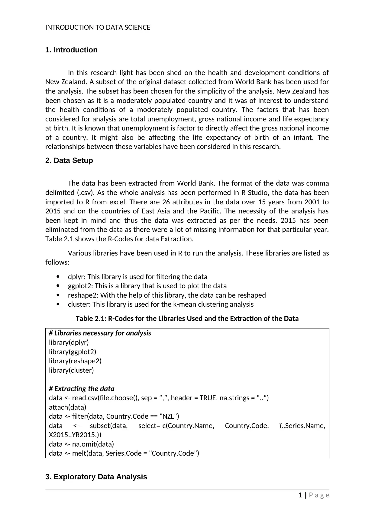
1. Introduction
In this research light has been shed on the health and development conditions of
New Zealand. A subset of the original dataset collected from World Bank has been used for
the analysis. The subset has been chosen for the simplicity of the analysis. New Zealand has
been chosen as it is a moderately populated country and it was of interest to understand
the health conditions of a moderately populated country. The factors that has been
considered for analysis are total unemployment, gross national income and life expectancy
at birth. It is known that unemployment is factor to directly affect the gross national income
of a country. It might also be affecting the life expectancy of birth of an infant. The
relationships between these variables have been considered in this research.
2. Data Setup
The data has been extracted from World Bank. The format of the data was comma
delimited (.csv). As the whole analysis has been performed in R Studio, the data has been
imported to R from excel. There are 26 attributes in the data over 15 years from 2001 to
2015 and on the countries of East Asia and the Pacific. The necessity of the analysis has
been kept in mind and thus the data was extracted as per the needs. 2015 has been
eliminated from the data as there were a lot of missing information for that particular year.
Table 2.1 shows the R-Codes for data Extraction.
Various libraries have been used in R to run the analysis. These libraries are listed as
follows:
dplyr: This library is used for filtering the data
ggplot2: This is a library that is used to plot the data
reshape2: With the help of this library, the data can be reshaped
cluster: This library is used for the k-mean clustering analysis
Table 2.1: R-Codes for the Libraries Used and the Extraction of the Data
# Libraries necessary for analysis
library(dplyr)
library(ggplot2)
library(reshape2)
library(cluster)
# Extracting the data
data <- read.csv(file.choose(), sep = ”,”, header = TRUE, na.strings = “..”)
attach(data)
data <- filter(data, Country.Code == "NZL")
data <- subset(data, select=-c(Country.Name, Country.Code, ï..Series.Name,
X2015..YR2015.))
data <- na.omit(data)
data <- melt(data, Series.Code = "Country.Code")
3. Exploratory Data Analysis
1 | P a g e
Paraphrase This Document
Need a fresh take? Get an instant paraphrase of this document with our AI Paraphraser
INTRODUCTION TO DATA SCIENCE
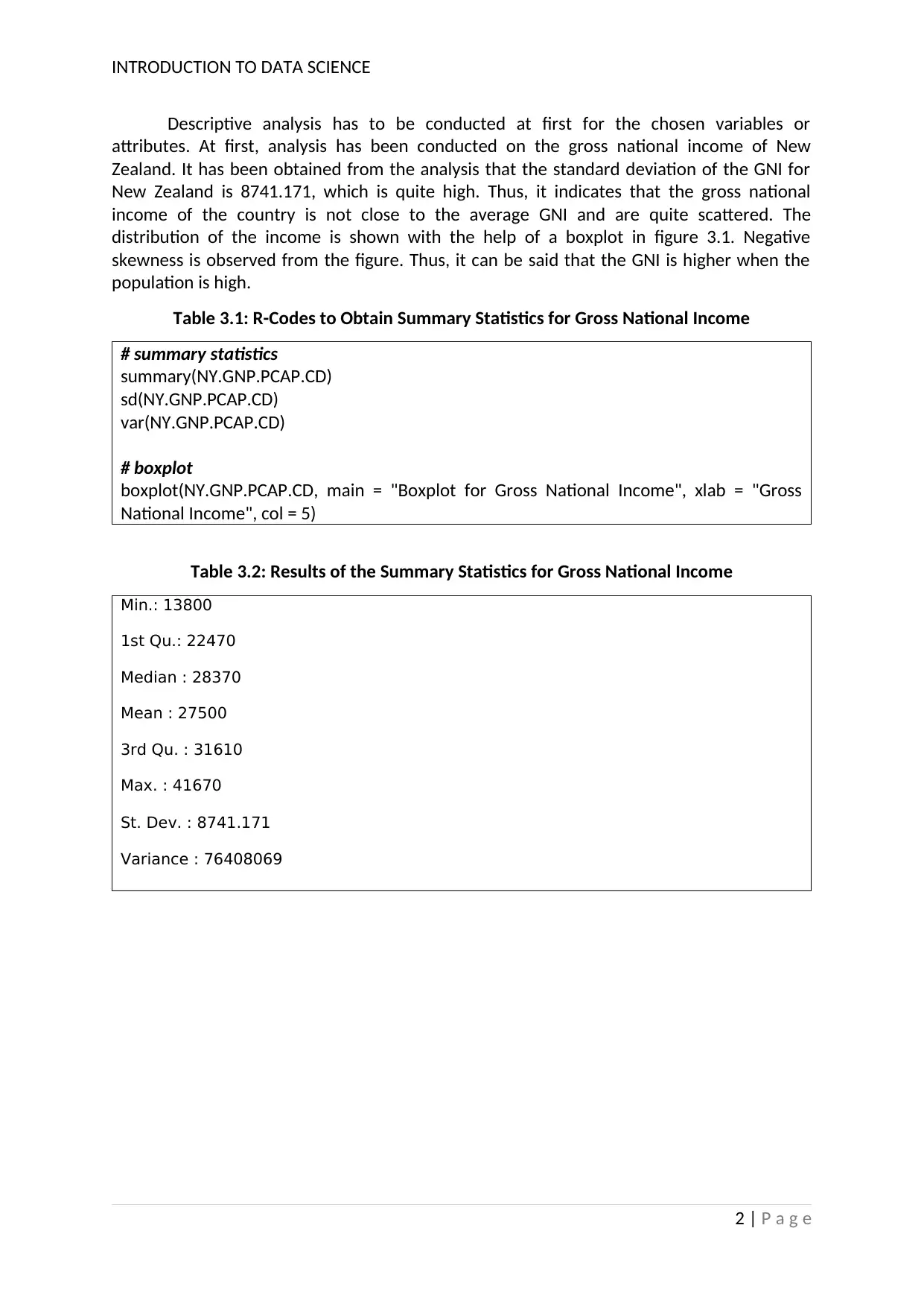
Descriptive analysis has to be conducted at first for the chosen variables or
attributes. At first, analysis has been conducted on the gross national income of New
Zealand. It has been obtained from the analysis that the standard deviation of the GNI for
New Zealand is 8741.171, which is quite high. Thus, it indicates that the gross national
income of the country is not close to the average GNI and are quite scattered. The
distribution of the income is shown with the help of a boxplot in figure 3.1. Negative
skewness is observed from the figure. Thus, it can be said that the GNI is higher when the
population is high.
Table 3.1: R-Codes to Obtain Summary Statistics for Gross National Income
# summary statistics
summary(NY.GNP.PCAP.CD)
sd(NY.GNP.PCAP.CD)
var(NY.GNP.PCAP.CD)
# boxplot
boxplot(NY.GNP.PCAP.CD, main = "Boxplot for Gross National Income", xlab = "Gross
National Income", col = 5)
Table 3.2: Results of the Summary Statistics for Gross National Income
Min.: 13800
1st Qu.: 22470
Median : 28370
Mean : 27500
3rd Qu. : 31610
Max. : 41670
St. Dev. : 8741.171
Variance : 76408069
2 | P a g e
INTRODUCTION TO DATA SCIENCE
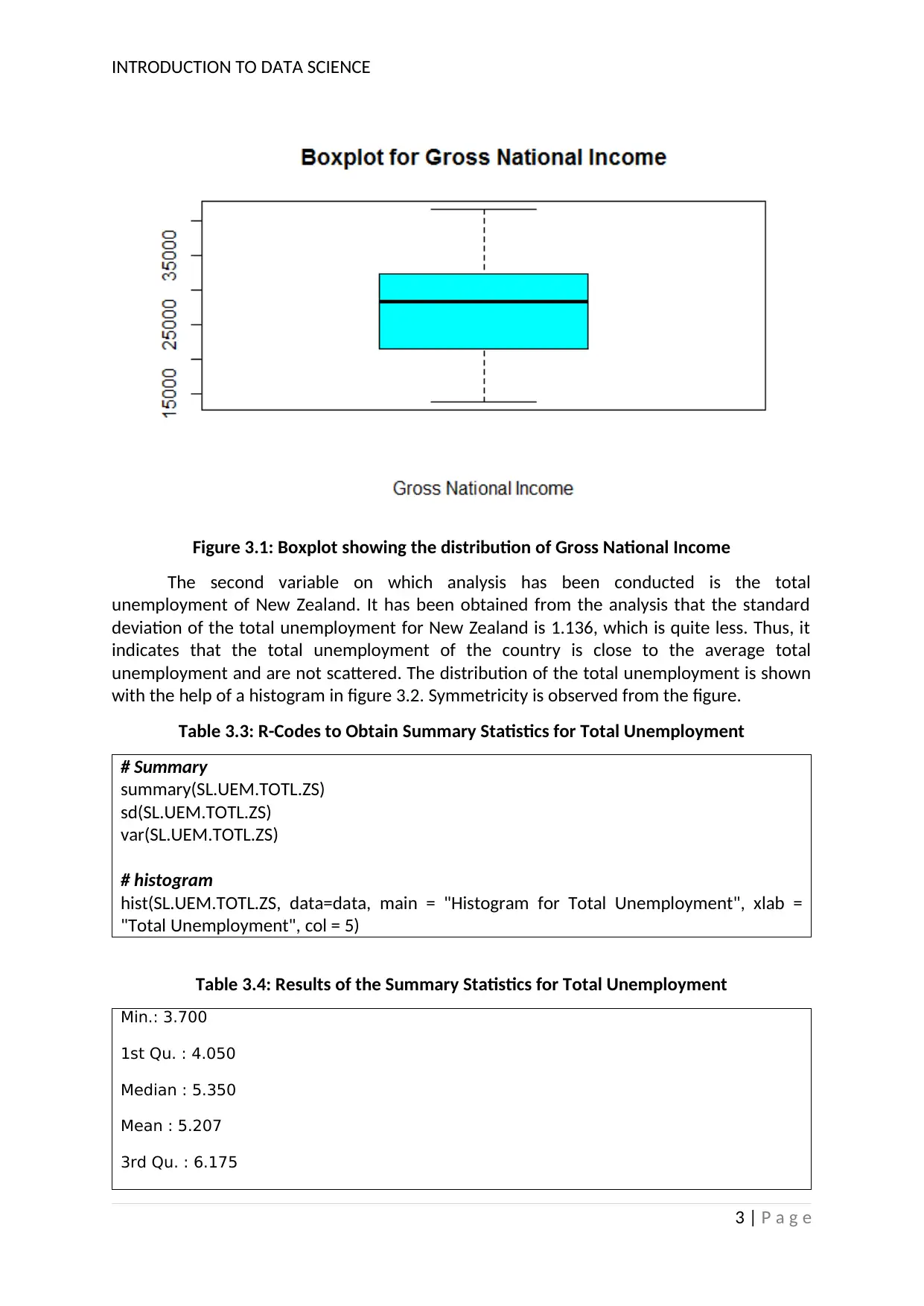
Figure 3.1: Boxplot showing the distribution of Gross National Income
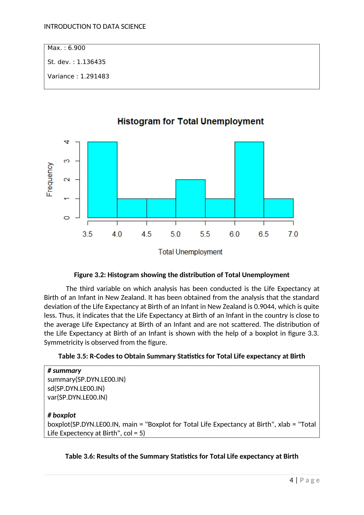
The second variable on which analysis has been conducted is the total
unemployment of New Zealand. It has been obtained from the analysis that the standard
deviation of the total unemployment for New Zealand is 1.136, which is quite less. Thus, it
indicates that the total unemployment of the country is close to the average total
unemployment and are not scattered. The distribution of the total unemployment is shown
with the help of a histogram in figure 3.2. Symmetricity is observed from the figure.
Table 3.3: R-Codes to Obtain Summary Statistics for Total Unemployment
# Summary
summary(SL.UEM.TOTL.ZS)
sd(SL.UEM.TOTL.ZS)
var(SL.UEM.TOTL.ZS)
# histogram
hist(SL.UEM.TOTL.ZS, data=data, main = "Histogram for Total Unemployment", xlab =
"Total Unemployment", col = 5)
Table 3.4: Results of the Summary Statistics for Total Unemployment
Min.: 3.700
1st Qu. : 4.050
Median : 5.350
Mean : 5.207
3rd Qu. : 6.175
3 | P a g e
Figure 3.1: Boxplot showing the distribution of Gross National Income
The second variable on which analysis has been conducted is the total
unemployment of New Zealand. It has been obtained from the analysis that the standard
deviation of the total unemployment for New Zealand is 1.136, which is quite less. Thus, it
indicates that the total unemployment of the country is close to the average total
unemployment and are not scattered. The distribution of the total unemployment is shown
with the help of a histogram in figure 3.2. Symmetricity is observed from the figure.
Table 3.3: R-Codes to Obtain Summary Statistics for Total Unemployment
# Summary
summary(SL.UEM.TOTL.ZS)
sd(SL.UEM.TOTL.ZS)
var(SL.UEM.TOTL.ZS)
# histogram
hist(SL.UEM.TOTL.ZS, data=data, main = "Histogram for Total Unemployment", xlab =
"Total Unemployment", col = 5)
Table 3.4: Results of the Summary Statistics for Total Unemployment
Min.: 3.700
1st Qu. : 4.050
Median : 5.350
Mean : 5.207
3rd Qu. : 6.175
3 | P a g e
⊘ This is a preview!⊘
Do you want full access?
Subscribe today to unlock all pages.
Trusted by 1+ million students worldwide
INTRODUCTION TO DATA SCIENCE
Max. : 6.900
St. dev. : 1.136435
Variance : 1.291483
Figure 3.2: Histogram showing the distribution of Total Unemployment
The third variable on which analysis has been conducted is the Life Expectancy at
Birth of an Infant in New Zealand. It has been obtained from the analysis that the standard
deviation of the Life Expectancy at Birth of an Infant in New Zealand is 0.9044, which is quite
less. Thus, it indicates that the Life Expectancy at Birth of an Infant in the country is close to
the average Life Expectancy at Birth of an Infant and are not scattered. The distribution of
the Life Expectancy at Birth of an Infant is shown with the help of a boxplot in figure 3.3.
Symmetricity is observed from the figure.
Table 3.5: R-Codes to Obtain Summary Statistics for Total Life expectancy at Birth
# summary
summary(SP.DYN.LE00.IN)
sd(SP.DYN.LE00.IN)
var(SP.DYN.LE00.IN)
# boxplot
boxplot(SP.DYN.LE00.IN, main = "Boxplot for Total Life Expectancy at Birth", xlab = "Total
Life Expectency at Birth", col = 5)
Table 3.6: Results of the Summary Statistics for Total Life expectancy at Birth
4 | P a g e
Paraphrase This Document
Need a fresh take? Get an instant paraphrase of this document with our AI Paraphraser
INTRODUCTION TO DATA SCIENCE
Min.: 78.69
1st Qu. : 79.62
Median : 80.25
Mean : 80.21
3rd Qu. : 80.85
Max. : 81.41
St. dev. : 0.9043788
Variance : 0.8179011
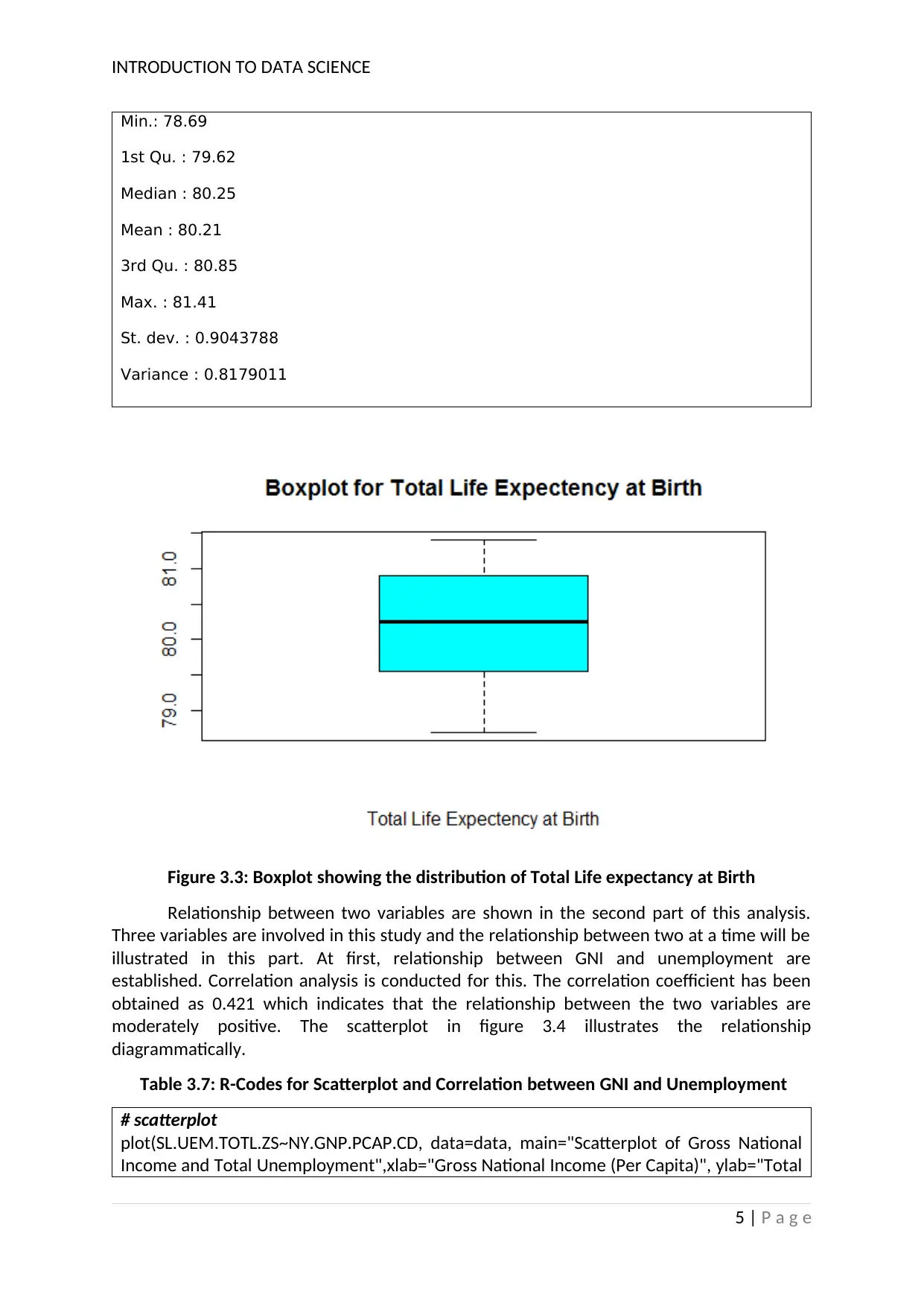
Figure 3.3: Boxplot showing the distribution of Total Life expectancy at Birth
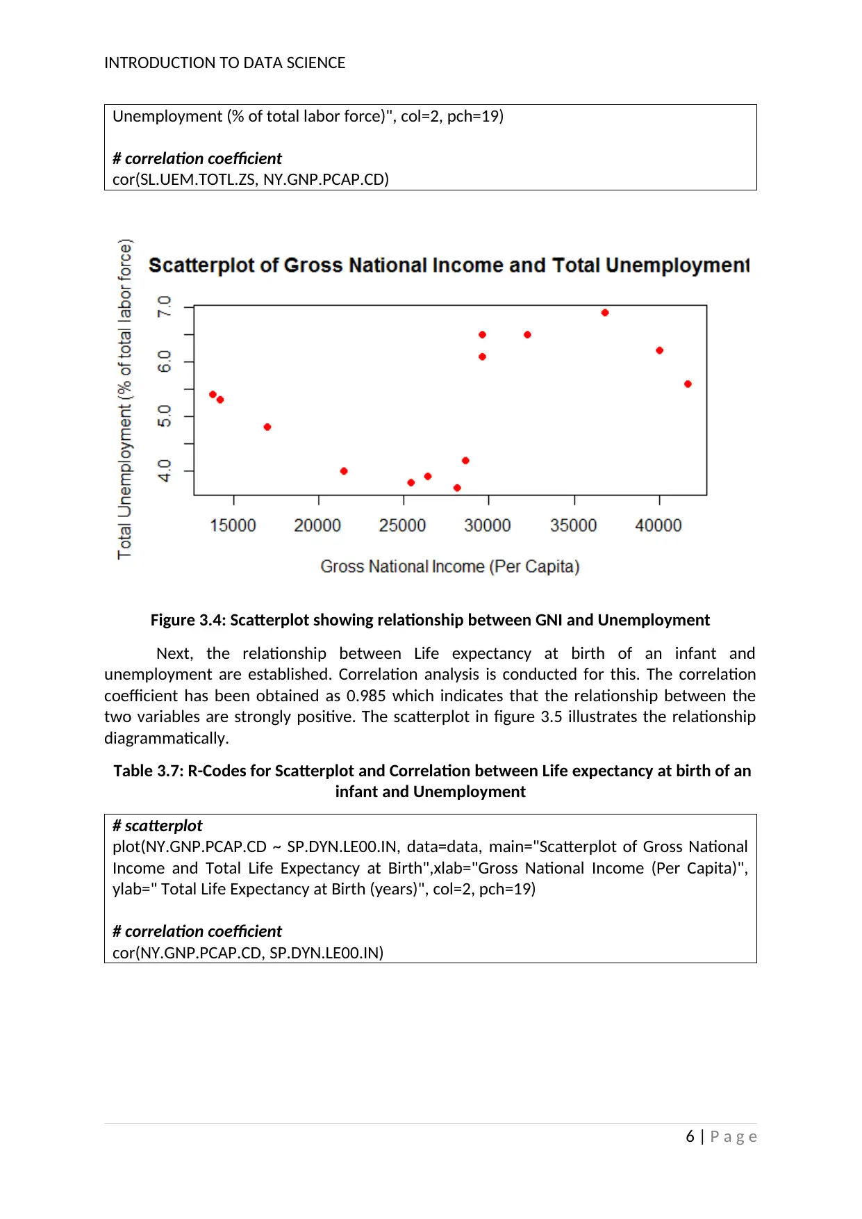
Relationship between two variables are shown in the second part of this analysis.
Three variables are involved in this study and the relationship between two at a time will be
illustrated in this part. At first, relationship between GNI and unemployment are
established. Correlation analysis is conducted for this. The correlation coefficient has been
obtained as 0.421 which indicates that the relationship between the two variables are
moderately positive. The scatterplot in figure 3.4 illustrates the relationship
diagrammatically.
Table 3.7: R-Codes for Scatterplot and Correlation between GNI and Unemployment
# scatterplot
plot(SL.UEM.TOTL.ZS~NY.GNP.PCAP.CD, data=data, main="Scatterplot of Gross National
Income and Total Unemployment",xlab="Gross National Income (Per Capita)", ylab="Total
5 | P a g e
Min.: 78.69
1st Qu. : 79.62
Median : 80.25
Mean : 80.21
3rd Qu. : 80.85
Max. : 81.41
St. dev. : 0.9043788
Variance : 0.8179011
Figure 3.3: Boxplot showing the distribution of Total Life expectancy at Birth
Relationship between two variables are shown in the second part of this analysis.
Three variables are involved in this study and the relationship between two at a time will be
illustrated in this part. At first, relationship between GNI and unemployment are
established. Correlation analysis is conducted for this. The correlation coefficient has been
obtained as 0.421 which indicates that the relationship between the two variables are
moderately positive. The scatterplot in figure 3.4 illustrates the relationship
diagrammatically.
Table 3.7: R-Codes for Scatterplot and Correlation between GNI and Unemployment
# scatterplot
plot(SL.UEM.TOTL.ZS~NY.GNP.PCAP.CD, data=data, main="Scatterplot of Gross National
Income and Total Unemployment",xlab="Gross National Income (Per Capita)", ylab="Total
5 | P a g e
INTRODUCTION TO DATA SCIENCE
Unemployment (% of total labor force)", col=2, pch=19)
# correlation coefficient
cor(SL.UEM.TOTL.ZS, NY.GNP.PCAP.CD)
Figure 3.4: Scatterplot showing relationship between GNI and Unemployment
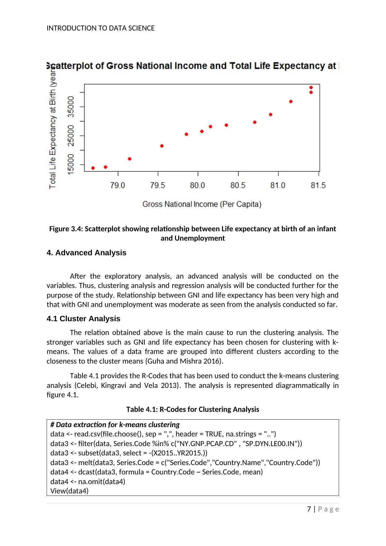
Next, the relationship between Life expectancy at birth of an infant and
unemployment are established. Correlation analysis is conducted for this. The correlation
coefficient has been obtained as 0.985 which indicates that the relationship between the
two variables are strongly positive. The scatterplot in figure 3.5 illustrates the relationship
diagrammatically.
Table 3.7: R-Codes for Scatterplot and Correlation between Life expectancy at birth of an
infant and Unemployment
# scatterplot
plot(NY.GNP.PCAP.CD ~ SP.DYN.LE00.IN, data=data, main="Scatterplot of Gross National
Income and Total Life Expectancy at Birth",xlab="Gross National Income (Per Capita)",
ylab=" Total Life Expectancy at Birth (years)", col=2, pch=19)
# correlation coefficient
cor(NY.GNP.PCAP.CD, SP.DYN.LE00.IN)
6 | P a g e
Unemployment (% of total labor force)", col=2, pch=19)
# correlation coefficient
cor(SL.UEM.TOTL.ZS, NY.GNP.PCAP.CD)
Figure 3.4: Scatterplot showing relationship between GNI and Unemployment
Next, the relationship between Life expectancy at birth of an infant and
unemployment are established. Correlation analysis is conducted for this. The correlation
coefficient has been obtained as 0.985 which indicates that the relationship between the
two variables are strongly positive. The scatterplot in figure 3.5 illustrates the relationship
diagrammatically.
Table 3.7: R-Codes for Scatterplot and Correlation between Life expectancy at birth of an
infant and Unemployment
# scatterplot
plot(NY.GNP.PCAP.CD ~ SP.DYN.LE00.IN, data=data, main="Scatterplot of Gross National
Income and Total Life Expectancy at Birth",xlab="Gross National Income (Per Capita)",
ylab=" Total Life Expectancy at Birth (years)", col=2, pch=19)
# correlation coefficient
cor(NY.GNP.PCAP.CD, SP.DYN.LE00.IN)
6 | P a g e
⊘ This is a preview!⊘
Do you want full access?
Subscribe today to unlock all pages.
Trusted by 1+ million students worldwide
INTRODUCTION TO DATA SCIENCE
Figure 3.4: Scatterplot showing relationship between Life expectancy at birth of an infant
and Unemployment
4. Advanced Analysis
After the exploratory analysis, an advanced analysis will be conducted on the
variables. Thus, clustering analysis and regression analysis will be conducted further for the
purpose of the study. Relationship between GNI and life expectancy has been very high and
that with GNI and unemployment was moderate as seen from the analysis conducted so far.
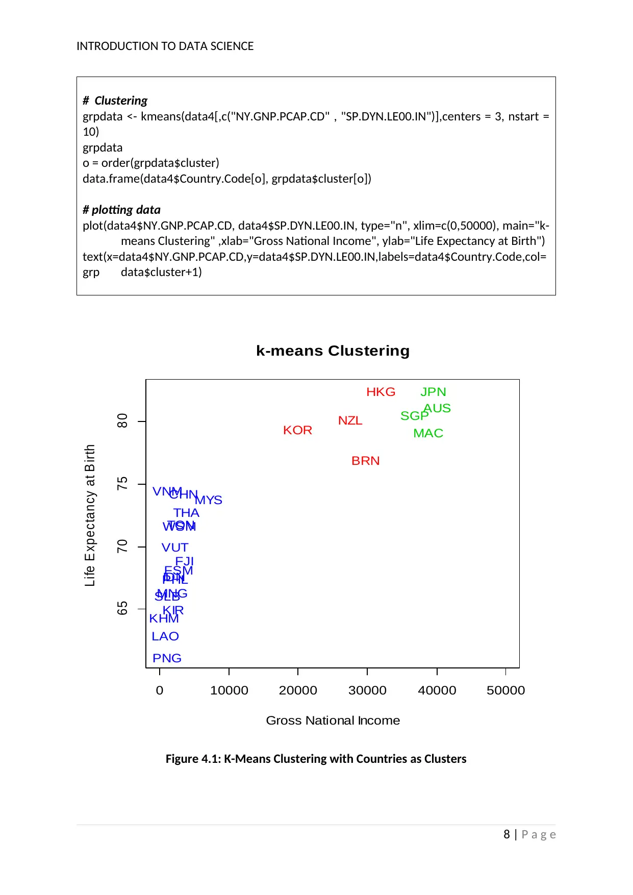
4.1 Cluster Analysis
The relation obtained above is the main cause to run the clustering analysis. The
stronger variables such as GNI and life expectancy has been chosen for clustering with k-
means. The values of a data frame are grouped into different clusters according to the
closeness to the cluster means (Guha and Mishra 2016).
Table 4.1 provides the R-Codes that has been used to conduct the k-means clustering
analysis (Celebi, Kingravi and Vela 2013). The analysis is represented diagrammatically in
figure 4.1.
Table 4.1: R-Codes for Clustering Analysis
# Data extraction for k-means clustering
data <- read.csv(file.choose(), sep = ",", header = TRUE, na.strings = "..")
data3 <- filter(data, Series.Code %in% c("NY.GNP.PCAP.CD" , "SP.DYN.LE00.IN"))
data3 <- subset(data3, select = -(X2015..YR2015.))
data3 <- melt(data3, Series.Code = c("Series.Code","Country.Name","Country.Code"))
data4 <- dcast(data3, formula = Country.Code ~ Series.Code, mean)
data4 <- na.omit(data4)
View(data4)
7 | P a g e
Figure 3.4: Scatterplot showing relationship between Life expectancy at birth of an infant
and Unemployment
4. Advanced Analysis
After the exploratory analysis, an advanced analysis will be conducted on the
variables. Thus, clustering analysis and regression analysis will be conducted further for the
purpose of the study. Relationship between GNI and life expectancy has been very high and
that with GNI and unemployment was moderate as seen from the analysis conducted so far.
4.1 Cluster Analysis
The relation obtained above is the main cause to run the clustering analysis. The
stronger variables such as GNI and life expectancy has been chosen for clustering with k-
means. The values of a data frame are grouped into different clusters according to the
closeness to the cluster means (Guha and Mishra 2016).
Table 4.1 provides the R-Codes that has been used to conduct the k-means clustering
analysis (Celebi, Kingravi and Vela 2013). The analysis is represented diagrammatically in
figure 4.1.
Table 4.1: R-Codes for Clustering Analysis
# Data extraction for k-means clustering
data <- read.csv(file.choose(), sep = ",", header = TRUE, na.strings = "..")
data3 <- filter(data, Series.Code %in% c("NY.GNP.PCAP.CD" , "SP.DYN.LE00.IN"))
data3 <- subset(data3, select = -(X2015..YR2015.))
data3 <- melt(data3, Series.Code = c("Series.Code","Country.Name","Country.Code"))
data4 <- dcast(data3, formula = Country.Code ~ Series.Code, mean)
data4 <- na.omit(data4)
View(data4)
7 | P a g e
Paraphrase This Document
Need a fresh take? Get an instant paraphrase of this document with our AI Paraphraser
INTRODUCTION TO DATA SCIENCE
# Clustering
grpdata <- kmeans(data4[,c("NY.GNP.PCAP.CD" , "SP.DYN.LE00.IN")],centers = 3, nstart =
10)
grpdata
o = order(grpdata$cluster)
data.frame(data4$Country.Code[o], grpdata$cluster[o])
# plotting data
plot(data4$NY.GNP.PCAP.CD, data4$SP.DYN.LE00.IN, type="n", xlim=c(0,50000), main="k-
means Clustering" ,xlab="Gross National Income", ylab="Life Expectancy at Birth")
text(x=data4$NY.GNP.PCAP.CD,y=data4$SP.DYN.LE00.IN,labels=data4$Country.Code,col=
grp data$cluster+1)
0 10000 20000 30000 40000 50000
65 70 75 80
k-means Clustering
Gross National Income
Life E xpectancy at B irth
AUS
BRN
CHN
FJI
FSM
HKG
IDN
JPN
KHM
KIR
KOR
LAO
MAC
MNG
MYS
NZL
PHL
PNG
SGP
SLB
THA
TON
VNM
VUT
WSM
Figure 4.1: K-Means Clustering with Countries as Clusters
8 | P a g e
INTRODUCTION TO DATA SCIENCE
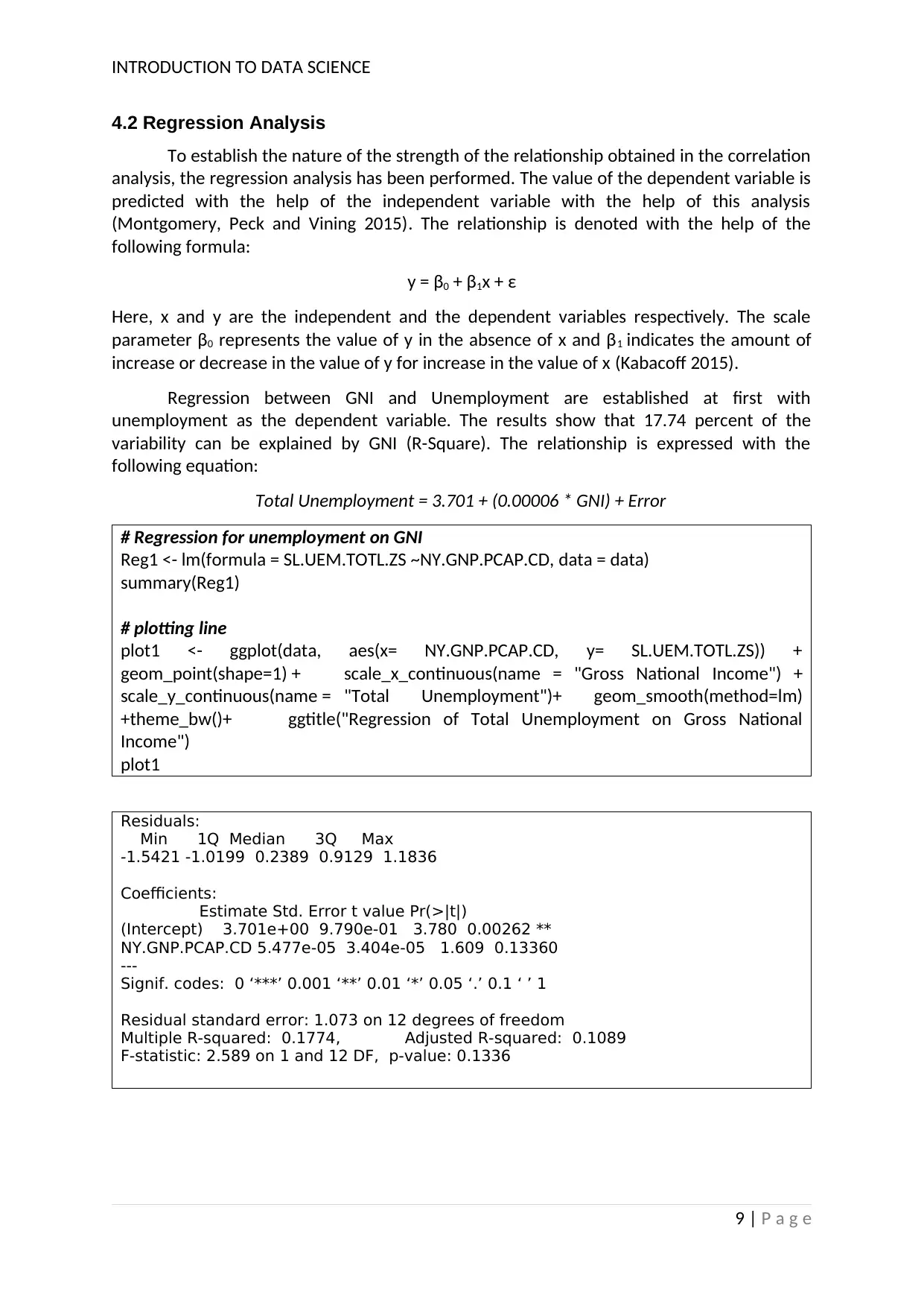
4.2 Regression Analysis
To establish the nature of the strength of the relationship obtained in the correlation
analysis, the regression analysis has been performed. The value of the dependent variable is
predicted with the help of the independent variable with the help of this analysis
(Montgomery, Peck and Vining 2015). The relationship is denoted with the help of the
following formula:
y = β0 + β1x + ε
Here, x and y are the independent and the dependent variables respectively. The scale
parameter β0 represents the value of y in the absence of x and β1 indicates the amount of
increase or decrease in the value of y for increase in the value of x (Kabacoff 2015).
Regression between GNI and Unemployment are established at first with
unemployment as the dependent variable. The results show that 17.74 percent of the
variability can be explained by GNI (R-Square). The relationship is expressed with the
following equation:
Total Unemployment = 3.701 + (0.00006 * GNI) + Error
# Regression for unemployment on GNI
Reg1 <- lm(formula = SL.UEM.TOTL.ZS ~NY.GNP.PCAP.CD, data = data)
summary(Reg1)
# plotting line
plot1 <- ggplot(data, aes(x= NY.GNP.PCAP.CD, y= SL.UEM.TOTL.ZS)) +
geom_point(shape=1) + scale_x_continuous(name = "Gross National Income") +
scale_y_continuous(name = "Total Unemployment")+ geom_smooth(method=lm)
+theme_bw()+ ggtitle("Regression of Total Unemployment on Gross National
Income")
plot1
Residuals:
Min 1Q Median 3Q Max
-1.5421 -1.0199 0.2389 0.9129 1.1836
Coefficients:
Estimate Std. Error t value Pr(>|t|)
(Intercept) 3.701e+00 9.790e-01 3.780 0.00262 **
NY.GNP.PCAP.CD 5.477e-05 3.404e-05 1.609 0.13360
---
Signif. codes: 0 ‘***’ 0.001 ‘**’ 0.01 ‘*’ 0.05 ‘.’ 0.1 ‘ ’ 1
Residual standard error: 1.073 on 12 degrees of freedom
Multiple R-squared: 0.1774, Adjusted R-squared: 0.1089
F-statistic: 2.589 on 1 and 12 DF, p-value: 0.1336
9 | P a g e
⊘ This is a preview!⊘
Do you want full access?
Subscribe today to unlock all pages.
Trusted by 1+ million students worldwide
1 out of 15
Related Documents


Your All-in-One AI-Powered Toolkit for Academic Success.
+13062052269
info@desklib.com
Available 24*7 on WhatsApp / Email
![[object Object]](/_next/static/media/star-bottom.7253800d.svg)
Unlock your academic potential
Copyright © 2020–2026 A2Z Services. All Rights Reserved. Developed and managed by ZUCOL.