Analysis of Bank Marketing Campaign using Data Science Techniques

This report presents a comprehensive data science analysis of a Portuguese bank's marketing campaign. The primary objective is to predict which existing customers are most likely to subscribe to a term deposit, thereby optimizing marketing efforts. The analysis utilizes a dataset derived from phone call-based marketing campaigns, encompassing 41,188 rows and 21 attributes. The methodology includes data representation, cleaning, and exploratory visualization using ggplot2. Five machine learning models (Naïve Bayes, Random Forest, SVM, C5.0 and Logistic Regression) are implemented for classification, with the Naïve Bayes model achieving the highest accuracy. The report provides detailed visualizations of key attributes, such as education, marital status, and campaign outcomes. The conclusion highlights the significance of various attributes in building predictive models and recommends the Naïve Bayes model for identifying potential customers based on their demographic and campaign interaction data, enabling the bank to make cost-effective marketing decisions. The report also includes R code used for the analysis.

Running head: FOUNDATIONS OF DATA SCIENCE
Foundations of Data Science
Students Name:
Student ID:
University Name:
Paper Code:

2Foundations of Data Science
Abstract
From the past analysis it has been observed that the Portuguese bank have seen a decline in the revenue,
thus the bank has decided to take required action accordingly. After different investigation and analysis the
reason behind the declination was observed to be that the clients were not depositing money to the bank as
frequently as they did before. Fixed deposit or term deposits helps any bank by investing in some other
marketing strategies so that the bank can gain profit by such steps. People opt for fixed deposits as the
deposit for a limited time period can give them a whole lot of money with interest for individual bank.
Thus the main purpose of the analysis is that the Portuguese bank want to identify if from the existing
customers who have the higher chances to subscribe for a term deposit and the bank would like to focus
marketing effort over such clients.
The data used in this analysis is totally related to a marketing campaign which was organized by the
Portuguese banking institution. The campaign was totally based on phone calls where the bank marketing
peoples arranged the campaign using phone calls. More than one contact were registered for the same client
in order to access the information weather the client will subscribe or not. In the dataset “y” attribute is the
target variable which says weather the customer subscribed to the term deposit or not.
Different analysis and visualization have been performed to understand the relationship with different
attributes and at the end data pre-processing and building model has been done using five different machine
learning models. The classification model with the highest accuracy will be taken for consideration.
At the end a conclusion will be concluded based on the analysis and the outcomes of each model to predict
the potential customer.

3Foundations of Data Science
Table of Contents
Abstract............................................................................................................................................................2
Introduction......................................................................................................................................................4
Data...................................................................................................................................................................4
Methods............................................................................................................................................................4
Data Representation...................................................................................................................................5
Unstructured to Structured data.................................................................................................................5
Data cleaning.............................................................................................................................................5
Missing value imputation..........................................................................................................................5
Data subset selection and/or subsampling.................................................................................................5
Exploratory visualization using ggplot2....................................................................................................5
Result and Discussion......................................................................................................................................6
Conclusion........................................................................................................................................................7
References.........................................................................................................................................................7
Appendix...........................................................................................................................................................8

4Foundations of Data Science
Introduction
With the recent advancement of technology, machine learning has a huge impact nowadays. Many
industries uses these technology in terms to gain benefit and also for customer satisfaction (Lantz, 2013).
The dataset used is from a bank which has been collected from a marketing campaign. The main goal for the
analysis is to predict using different machine learning algorithm weather the bank customers will subscribe
to the bank deposit or not (Elsalamony, 2014). In the analysis five different machine learning algorithms has
been implemented which helps the marketing team to identify potential customers who are relatively more
likely to subscribe to the term deposit and this increase the hit ratio (Parlar & Acaravci, 2017).
Data
The dataset has been taken from
https://bigml.com/user/totyb/gallery/dataset/5092da63035d075cd100006c
A total of 41188 rows are there in the dataset with 21 numbers of attributes. A details information
about all the attributes will be described below.
Bank client data: The information relates to the demographic profile of the customers. In addition
information is also given for credit default, loan, housing and personal of the clients.
Related with the last contact of the current campaign: The information relates to the medium of contacts
which was last done in the previous campaign to every potential customer. This include contact mode, day
of weeks, duration etc.
Other attributes: The information relates to the number of contact, pdays, previous year’s campaign previous
total number of contacts counted.
Output variable (desired target): y - Has the client subscribed a term deposit? (binary: 'yes', 'no')
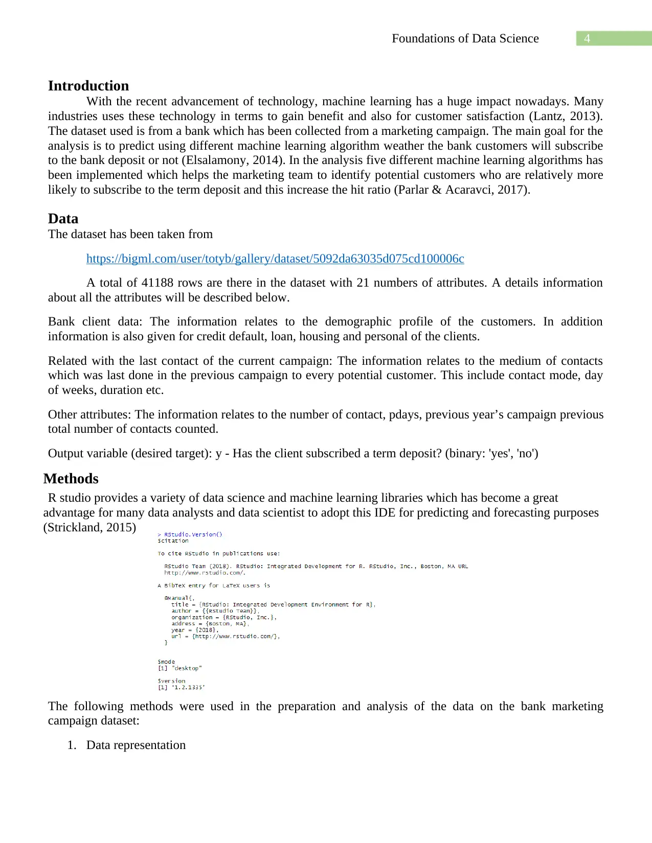
Methods
R studio provides a variety of data science and machine learning libraries which has become a great
advantage for many data analysts and data scientist to adopt this IDE for predicting and forecasting purposes
(Strickland, 2015)
The following methods were used in the preparation and analysis of the data on the bank marketing
campaign dataset:
1. Data representation

5Foundations of Data Science
2. Unstructured to Structured data
3. Data cleaning
4. Missing value imputation
5. Data subset selection and/or subsampling
6. Exploratory visualization using ggplot2
Data Representation: The dataset which is the Bank Marketing dataset which contains both numerical and
categorical variables. Also not all the attributes are essential for the analysis thus from the dataset 19
attributes from the 20 attributes excluding the target attributes are useful for prediction of future Term
Deposit subscriptions.
Unstructured to Structured data: The dataset used is a balanced dataset where it is easily understood by
machine language. The data is well maintained and properly structures. The dataset contains both numerical
and categorical values and the target variable is contains binary values either yes or no
Data cleaning: The dataset contains a lot of unknown values all over the attributes. No data cleaning has
been done since there are no missing values.
Missing value imputation: From the figure 1 it can be seen that that there are no missing or null values in
the dataset.
Data subset selection and/or subsampling: For machine learning model, the dataset have been divided
into 80-20 ratio of training and testing (Ramasubramanian & Singh, 2017). For model building 1000
samples are taken from the complete data set.
Figure 1: Missing value or null value percentage
Exploratory visualization using ggplot2: In the exploratory data visualization, the ggplot ( ) function from
the ggplot2 package was used. The exploratory data visualization plotted the age, education, job, housing,
loan, contacts and many other attributes details has been shown visually.
Result and Discussion

6Foundations of Data Science
Figure 2: Count for educational details
The results of the exploratory data visualization are as given from figure 1 to figure 5.
From the analysis and from figure 2 there are a total of 4.20268 % of cases labelled as unknown in
Education column in this results set.
Figure 3: Count Weather subscribed or not
Figure 3 shows the amount of customer subscribed for the loan and it’s clear that majority of the
customers did not subscribed.
Figure 4: count per month
A good bunch of campaign was done in Month of May. While the least was December, March,
October and September.

7Foundations of Data Science
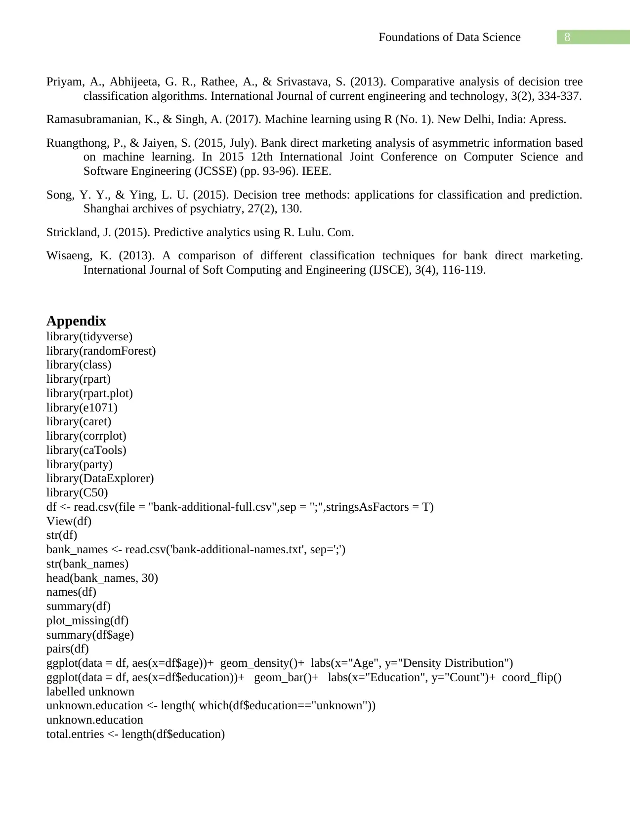
Figure 5: count of Outcome from previous campaign
Majority of campaign made seemingly resulted from persons who had non-existent status meaning it
was their first time, this is seen also in previous visualization of previous and pdays.
Conclusion
From the above analysis it can be concluded that the results are convincing and impressing side by
side by using machine learning algorithms to decide on the marketing campaign of the bank. Most of the
attributes in the dataset are significant for building the predictive model. Among all the five classification
algorithm Naïve Bayes model yielded the best accuracy of 94.47% accuracy level which is considered to be
a good model for the dataset. This model is simple and easy to implement.
Thus now the bank marketing manager will use the naïve Bayes model to identify potential
customers if the customer information like education, duration of the call, number of contacts performed
during this campaign, Personal loan, previous outcomes, housing loan, etc. is made available. By using such
data banks will be able to make critical decision over cost optimization by avoiding useless call to other
customers.
References
Bharathidason, S., & Venkataeswaran, C. J. (2014). Improving classification accuracy based on random
forest model with uncorrelated high performing trees. Int. J. Comput. Appl, 101(13), 26-30.
Biau, G., & Scornet, E. (2016). A random forest guided tour. Test, 25(2), 197-227.
Elsalamony, H. A. (2014). Bank direct marketing analysis of data mining techniques. International Journal
of Computer Applications, 85(7), 12-22.
Elsalamony, H. A., & Elsayad, A. M. (2013). Bank direct marketing based on neural network and C5. 0
Models. International Journal of Engineering and Advanced Technology (IJEAT), 2(6).
Ghosh, S., Hazra, A., Choudhury, B., Biswas, P., & Nag, A. (2018, July). A comparative study to the bank
market prediction. In International Conference on Machine Learning and Data Mining in Pattern
Recognition (pp. 259-268). Springer, Cham.
Lantz, B. (2013). Machine learning with R. Packt Publishing Ltd.
Lantz, B. (2019). Machine Learning with R: Expert techniques for predictive modeling. Packt Publishing
Ltd.
Parlar, T., & ACARAVCI, S. K. (2017). Using data mining techniques for detecting the important features
of the bank direct marketing data. International Journal of Economics and Financial Issues, 7(2),
692-696.
Patil, S. S., Patidar, K., & Jain, M. (2016). Stock market prediction using support vector machine.
International Journal of Current Trends in Engineering & Technology, 2(1), 18-25.

8Foundations of Data Science
Priyam, A., Abhijeeta, G. R., Rathee, A., & Srivastava, S. (2013). Comparative analysis of decision tree
classification algorithms. International Journal of current engineering and technology, 3(2), 334-337.
Ramasubramanian, K., & Singh, A. (2017). Machine learning using R (No. 1). New Delhi, India: Apress.
Ruangthong, P., & Jaiyen, S. (2015, July). Bank direct marketing analysis of asymmetric information based
on machine learning. In 2015 12th International Joint Conference on Computer Science and
Software Engineering (JCSSE) (pp. 93-96). IEEE.
Song, Y. Y., & Ying, L. U. (2015). Decision tree methods: applications for classification and prediction.
Shanghai archives of psychiatry, 27(2), 130.
Strickland, J. (2015). Predictive analytics using R. Lulu. Com.
Wisaeng, K. (2013). A comparison of different classification techniques for bank direct marketing.
International Journal of Soft Computing and Engineering (IJSCE), 3(4), 116-119.
Appendix
library(tidyverse)
library(randomForest)
library(class)
library(rpart)
library(rpart.plot)
library(e1071)
library(caret)
library(corrplot)
library(caTools)
library(party)
library(DataExplorer)
library(C50)
df <- read.csv(file = "bank-additional-full.csv",sep = ";",stringsAsFactors = T)
View(df)
str(df)
bank_names <- read.csv('bank-additional-names.txt', sep=';')
str(bank_names)
head(bank_names, 30)
names(df)
summary(df)
plot_missing(df)
summary(df$age)
pairs(df)
ggplot(data = df, aes(x=df$age))+ geom_density()+ labs(x="Age", y="Density Distribution")
ggplot(data = df, aes(x=df$education))+ geom_bar()+ labs(x="Education", y="Count")+ coord_flip()
labelled unknown
unknown.education <- length( which(df$education=="unknown"))
unknown.education
total.entries <- length(df$education)

9Foundations of Data Science
cat("There are a total of ",(unknown.education/total.entries)*100,"% of cases labelled as unknown in
Education collumn in this results set")
ggplot(data = df, aes(x=df$marital))+ geom_bar()+ labs(x="Marital Status", y="Count")
cat("Cases of unknown is also distributed in Marriage category forming",
(length(which(df$marital=="unknown"))/total.entries)*100,"% of the total studied population")
ggplot(data = df, aes(x=df$marital))+ geom_bar()+ labs(x="Marital Status", y="Count")
cat("Cases of unknown is also distributed in Marriage category forming",
(length(which(df$marital=="unknown"))/total.entries)*100,"% of the total studied population")
ggplot(data = df, aes(x=df$job))+ geom_bar()+ labs(x="Job Category", y="Count")+ coord_flip()
cat("Cases of unknown is also distributed in Job category forming",
(length(which(df$job=="unknown"))/total.entries)*100,"% of the total studied population")
ggplot(data = df, aes(x= df$default))+ geom_bar()+ labs(x="Credit Default", y="Count")
cat("Only ",length(which(df$default=="yes"))," cases have been reported for positive credit defaulters. This
is minimal and hence no significant effect to the final decision")
ggplot(data = df, aes(x=df$housing))+ geom_bar()+ labs(x="Housing", y="Count")
cat("There were ",length(which(df$housing=="unknown"))," cases have been reported for housing. This is
also minimal and hence no significant effect to the final decision")
ggplot(data = df, aes(x=df$loan))+ geom_bar()+ labs(x="Loan", y="Count")
cat("Evidently, majority of the group studied did not borrow loans. This contributed ",
(length(which(df$loan=="no"))/total.entries) * 100,"%. This is significant.")
ggplot(data = df, aes(x=df$loan, fill=df$y))+ labs(x="Loan", y="Count", fill="Subscribed?")+
geom_bar()
ggplot(data = df, aes(x=df$contact, fill=df$contact))+ geom_bar()+
labs(x="Contact", y="Count", fill="Contact Mode")
ggplot(data = df, aes(x=df$month, fill=df$month))+ geom_bar()+
labs(x="Month", y="Count", fill="Campaing Month")
ggplot(data = df, aes(x = df$day_of_week, fill=df$day_of_week))+ geom_bar()+
labs(x="Day of the Week", y="Count", fill="Day of the Week")
ggplot(data = df, aes(x=df$duration))+ geom_bar(position = "dodge")+ labs(x="Duration (seconds)",
y="count")
summary(df$duration)
plot_density(df$duration)
group_by
ggplot(data = df, aes(x=df$campaign))+ geom_bar()+ labs(x="Number of Campaings")+
scale_x_continuous(breaks=seq(0,30,2))
ggplot(data = df, aes(x=df$pdays))+ geom_histogram(bins=30)+ labs(x="Number of days since last
contact", y="Count")
ggplot(data = df, aes(x=df$previous))+ geom_histogram(bins=30)+labs(x="Contacts/Calls Made",
y="Count")
unique(df$poutcome)
ggplot(data = df, aes(x=df$poutcome, fill=df$y))+
geom_bar()+ labs(x="Outcome from previous campaing", y="count", fill="variable Y")
set.seed(150)
sample1 <-df[sample(nrow(df),1000), ]
partitioned <- createDataPartition( sample1$y, times = 1, p = 0.8, list = F)
train = sample1[partitioned, ]

10Foundations of Data Science
test = sample1[-partitioned, ]
prop.table(table(train$y))
prop.table(table(test$y))
ncol(train)
ncol(test)
dct <- C5.0(train[-21], as.factor(train$y))
summary(dct)
predict <- predict(dct,test)
confusionMatrix(as.factor(test$y), predict)
rm <- randomForest(train[-21], as.factor(train$y))
summary(rm)
predict <- predict(rm,test)
confusionMatrix(as.factor(test$y),predict)
svm <- svm(as.factor(train$y)~ ., data = train, kernel="linear")
summary(svm)
predict <- predict(svm, train[-21])
confusionMatrix(as.factor(train$y), predict)
naive.sample.train.model <- naiveBayes(train, train$y)
predict <- predict(naive.sample.train.model, test)
confusionMatrix(test$y, predict)
logistic = glm(y ~ .,data = train,family = "binomial")
suppressWarnings({logistic_train_score = predict(logistic,
newdata = train,
type = "response")})
suppressWarnings({logistic_test_score = predict(logistic,
newdata = test,
type = "response")})
logistic_train_cut = 0.2
fun_cut_predict = function(score, cut) {
classes = score
classes[classes > cut] = 1
classes[classes <= cut] = 0
classes = as.factor(classes)
return(classes) }
logistic_train_class = fun_cut_predict(logistic_train_score, logistic_train_cut)
predict_class <- factor(ifelse(logistic_train_class == 1, "yes", "no"))
confusionMatrix(predict_class, train$y, positive= "no")