Data Science Assignment on Statistical Analysis and R Programming

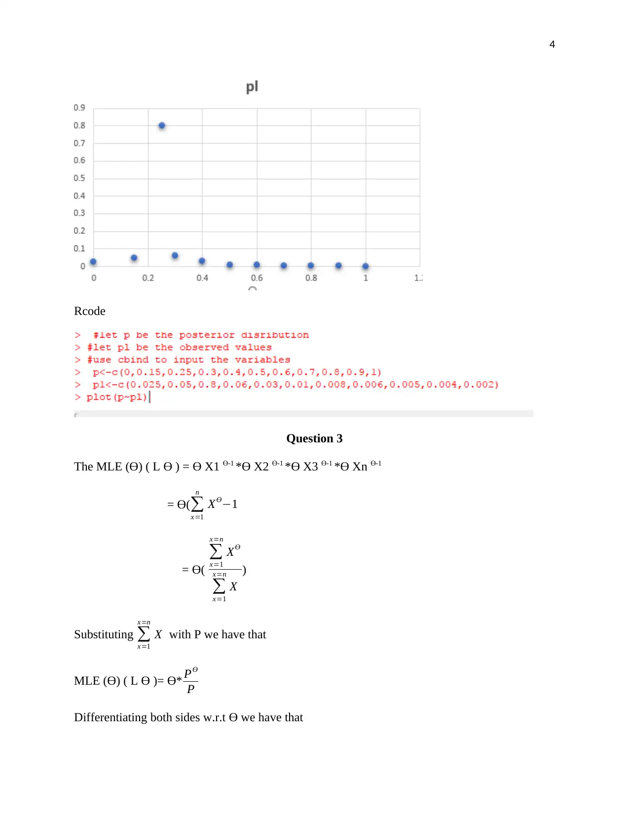
This data science assignment solution addresses several statistical concepts and their practical application using R programming. The assignment begins with the analysis of a random variable's distribution, calculating the distribution of a new variable derived from it. It then explores the expected value of a binomial distribution and provides R code to calculate it. The solution further delves into posterior distributions, estimation, and plotting. The document then examines Maximum Likelihood Estimation (MLE), deriving the MLE for a given function and analyzing how the variance changes with increasing values. Finally, the solution covers the Poisson probability distribution, calculating the MLE for the Poisson distribution and provides the necessary formulas and steps to derive the solution. The assignment includes citations for the references used.

1
Data Science
Student’s Name
Affiliation
Course
Instructor
Date

2
Question 1
A random variable V has a density fv(v) =Kv2 exp(-b/v2 )
a) What is the distribution of a new random variable, Y=1/2 mV2
The first step will entail differentiation of the function fv(v) =Kv2 exp(-b/v2 ) w.r.t V
d (f ( v ))
d(v ) =2KV* exp (-b/v2) + KV2*-2e-bv-3
The distribution for the new variable is given by
F(y)= 2KV* exp (-b/v2) + KV2*-2e-bv-3
b) in order to get the mean of y one has to differentiate y with respect to V and get the
d (f ( y ) )
d( y) = MV
The mean of Y=MV
Question 2
Que. A
> # the expected value of a binomial distribution is given by np
> #n is the number of observations
> #p is the number of success
> #p=6/10
> #n=10
> #let expected value be represented by M
> p<-6/10
> n<-10
> M<-p*n
> M

3
[1] 6
> #this means that the mean is 6
Rcode:
Que B
The posterior distribution is given by
P(Ɵ) ={ p=3/5 for x=1,2…..10
The estimated value for (Ɵ) is =Ɵ/6 where 6 is the mean of the distribution
Que. C
> p<-c(0,0.15,0.25,0.3,0.4,0.5,0.6,0.7,0.8,0.9,1)
> p1<-c(0.025,0.05,0.8,0.06,0.03,0.01,0.008,0.006,0.005,0.004,0.002)
> plot(p~pl)

4
Rcode
Question 3
The MLE (Ɵ) ( L Ɵ ) = Ɵ X1 Ɵ-1 *Ɵ X2 Ɵ-1 *Ɵ X3 Ɵ-1 *Ɵ Xn Ɵ-1
= Ɵ(∑
x=1
n
XƟ−1
= Ɵ(
∑
x=1
x=n
XƟ
∑
x=1
x=n
X
)
Substituting ∑
x=1
x=n
X with P we have that
MLE (Ɵ) ( L Ɵ )= Ɵ* PƟ
P
Differentiating both sides w.r.t Ɵ we have that

5
d (L (Ɵ ))
d (Ɵ) = 1* ƟP^Ɵ-2
Ɵ=¿ ƟP^Ɵ-2
Dividing both sides by Ɵ
1=P^Ɵ/P^2
P^2= P^Ɵ
2logP= Ɵ log P
Dividing both sides by log P
Ɵ=2
b) the MLE (Ɵ) ( L Ɵ )= Ɵ* PƟ
P
P is given by ∑
x=1
x=n
X
As the value of X increases it means that since Ɵ is fixed, the variance will decrease.
Question 4
a) The poison probability distribution is given by:
P(X:u)= ( e−u )∗(ux)
x ! , where x=1,2,3…n where u is the mean and x is the observed variable
P(Xi=x/X1=1) = P ¿ ¿ = e−i
e 1 . since the base for the denominator is equal to the base for the
numerator, then the equation is simplified into
P(Xi=x/X1=1) = e−i−1
b) The MLE is computed by getting the product of observable outcomes (Smirnov, 2011).
In this case one should multiply the function for all values of x in order to get a joint
distribution function

6
L(U) = ( e−u )∗(ux1 )
x 1! * ( e−u )∗(ux 2)
x 2 ! * ( e−u )∗(ux3 )
x 3 ! *… ( e−u )∗(uxi )
xi! (A’Hearn, 2004)
=e-nu(∑
i=1
n
ux / x !)
Taking differential from both sides the results are:
d (L (u ))
d (u) = -u* e-nu *(∑
i=1
n
ux / x !)
It therefore follows that the first part of the differentiation gives 1-e-u while the second
part gives ∑ ixi /n. Combining the two parts, the results for MLE becomes
Ǔ= 1-e-u *∑ ixi /n.
Substituting ∑ ixi /n with ẍ then the results becomes
Ǔ=1-e-u * ẍ
c) When ẍ= 3.2,the value for Ǔ is given by
Ǔ= 3.2* (1-e- Ǔ )
Ǔ
3.2 + e- Ǔ =1
Ǔ +3.2 e−Ǔ
3.2 =1
The value of u=0 for the equation above to be satisfied.
If zero replaces u the equation becomes
0+3.2 e−0
3.2 =1
Since any number raise to the power of zero=1, then
0+3.2
3.2 =1 which confirms that the value of Ǔ =0

7
Bibliography
A’Hearn, B., (2004). A restricted maximum likelihood estimator for truncated height
samples. Economics & Human Biology, 2(1), pp.5-19. (A’Hearn, 2004)
Smirnov, O., (2011). Maximum Likelihood Estimator for Multivariate Binary Response
Models. SSRN Electronic Journal,. (Smirnov, 2011)