Data Science: Regression, Classification, and Model Evaluation

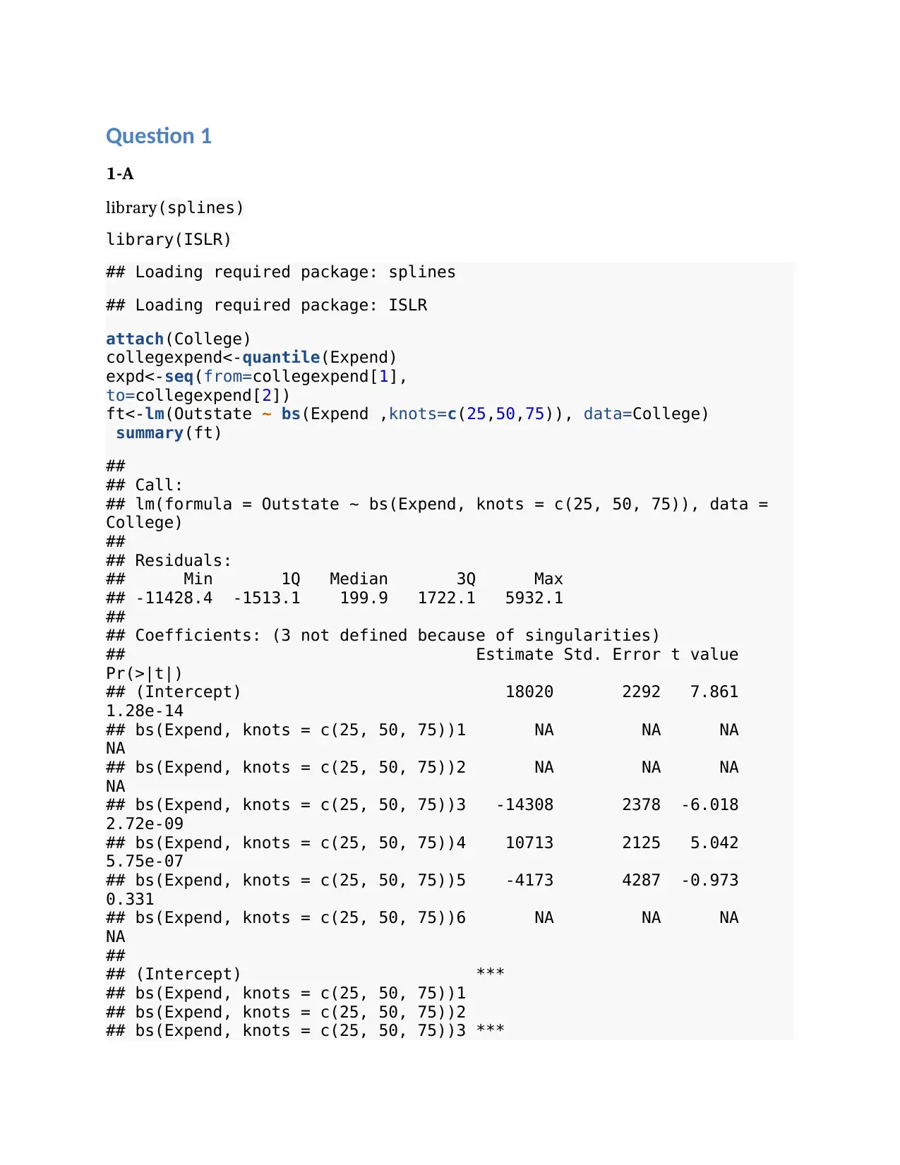
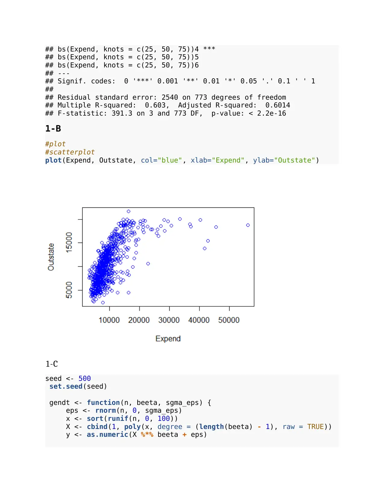
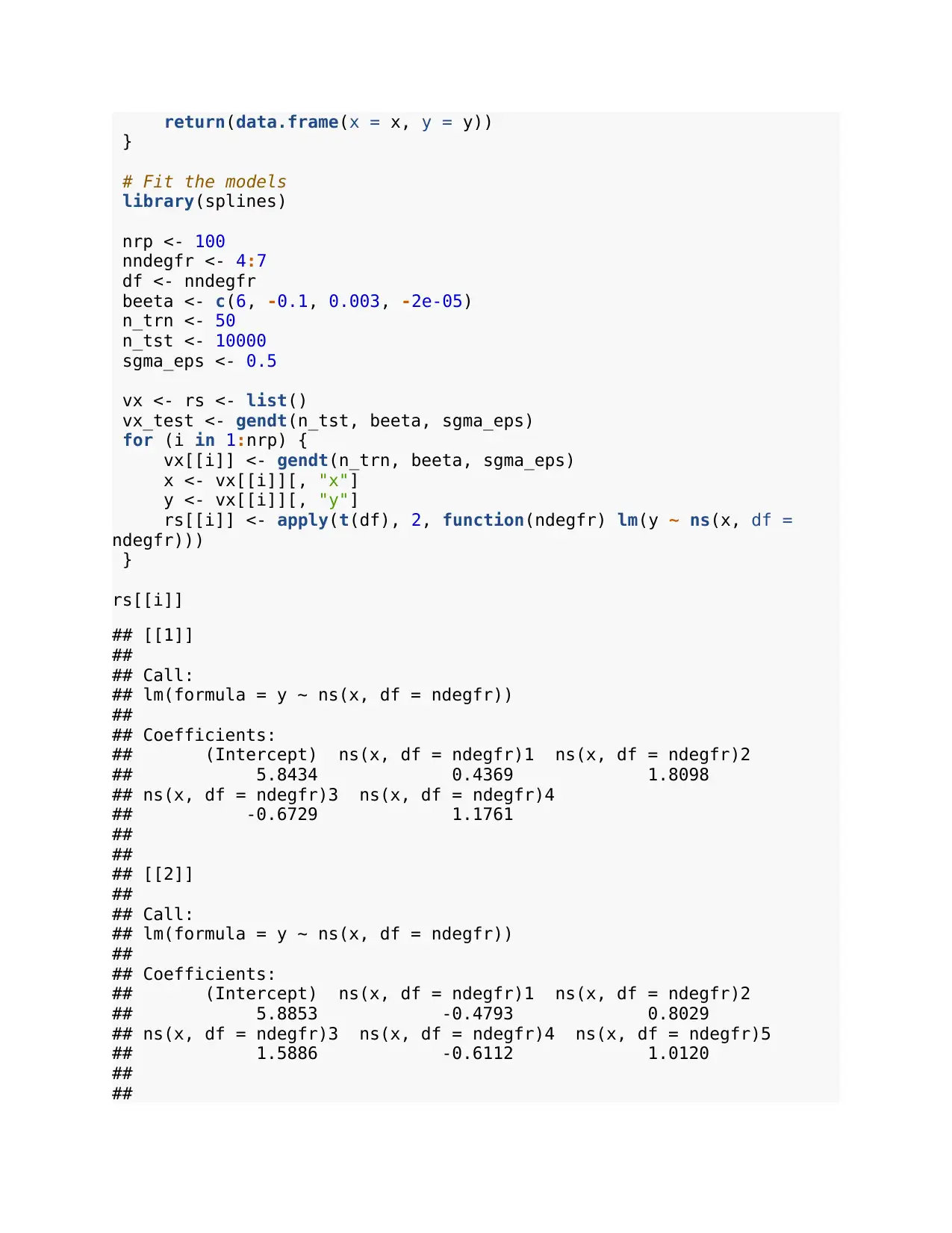
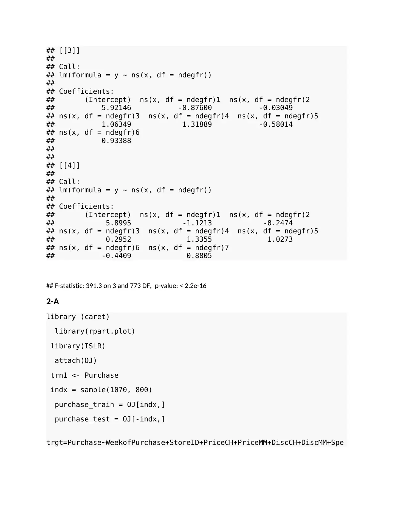
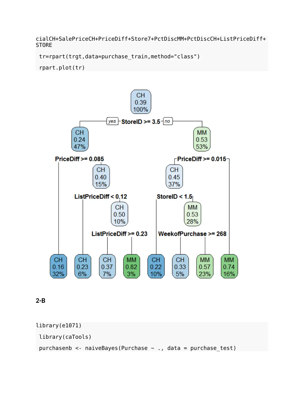
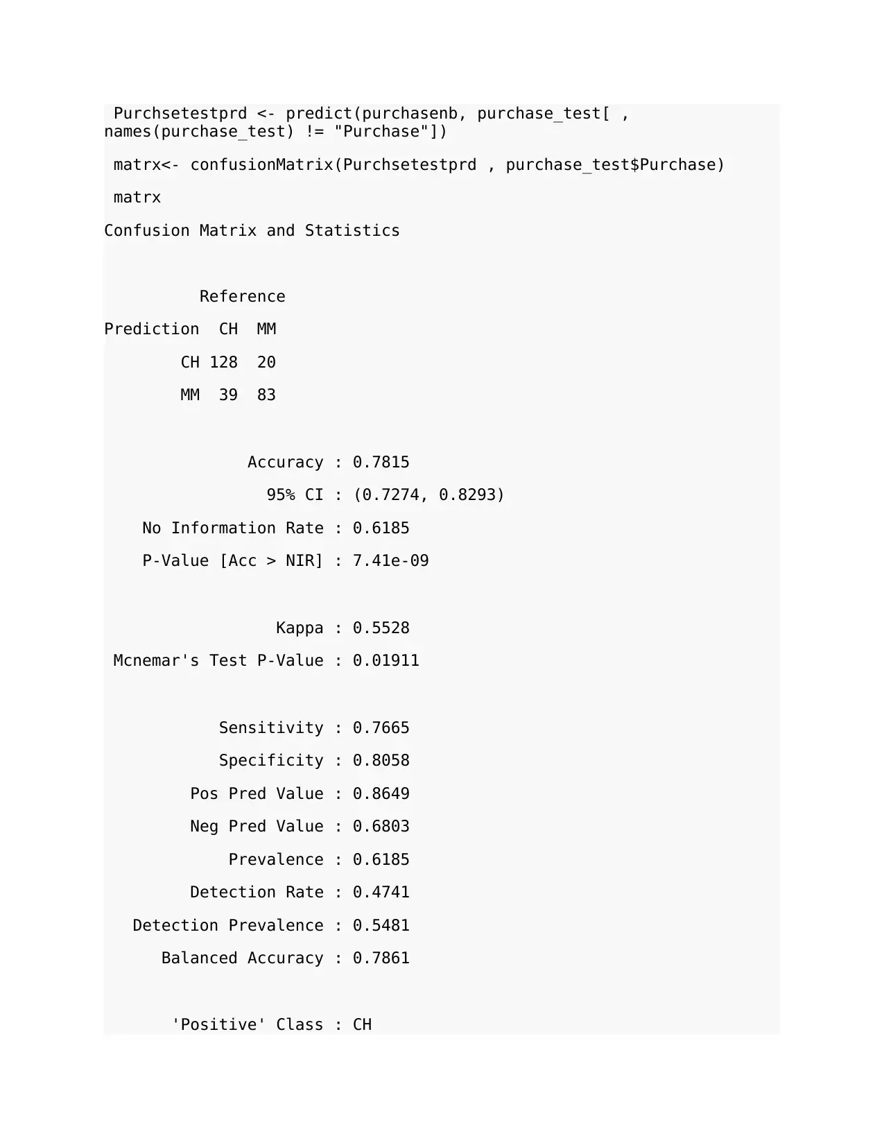
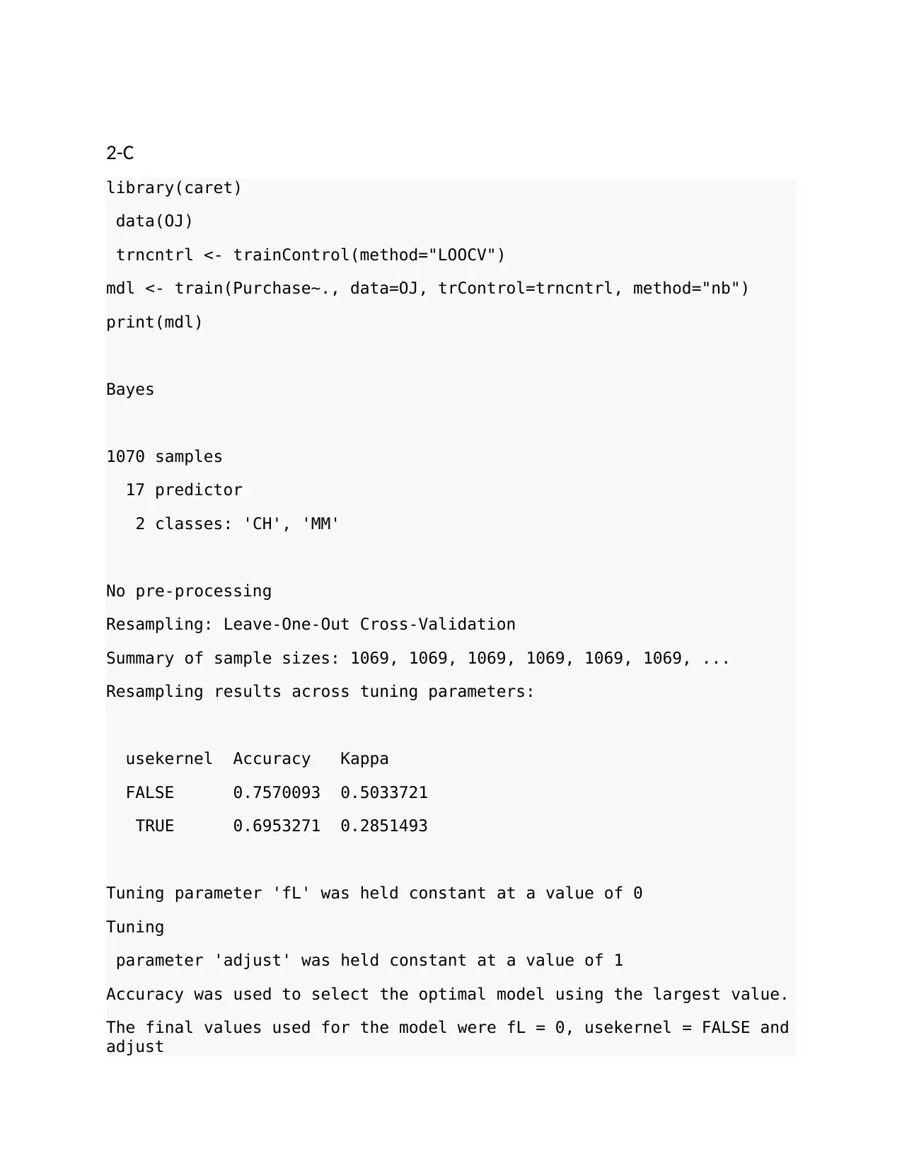
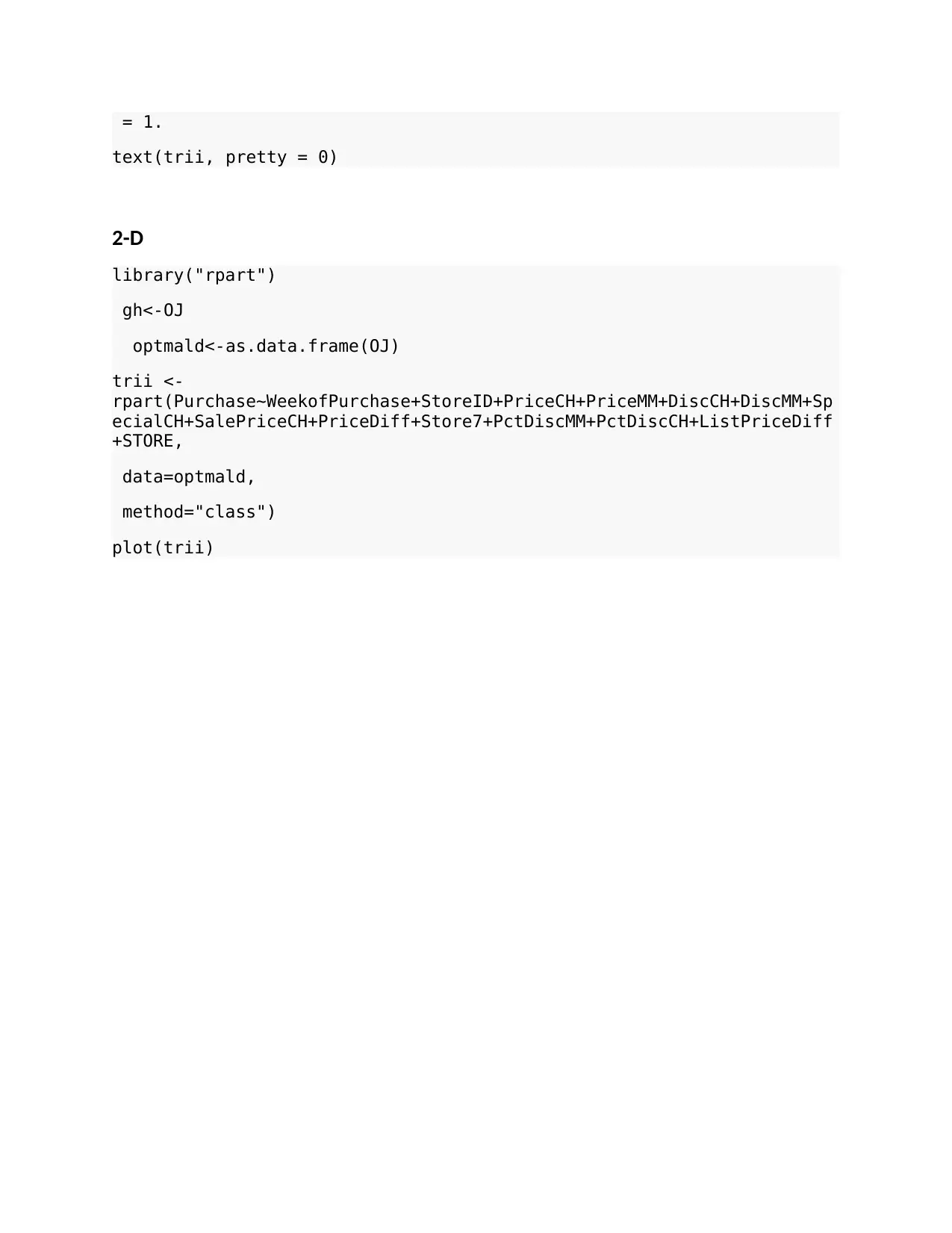
This assignment delves into various aspects of data science, encompassing regression analysis, classification models, and model evaluation techniques. The first part focuses on regression using splines, exploring model fitting, plotting, and cross-validation to assess model performance. The second part shifts to classification, utilizing decision trees, naive Bayes, and random forests to predict a binary outcome. The third part explores model selection and evaluation using cross-validation and lasso regression to refine the model's accuracy. The assignment includes code implementations, model summaries, and performance metrics to compare and contrast different approaches, providing a comprehensive understanding of data science methodologies. This assignment provides a practical exploration of various data science techniques including regression, classification, and model evaluation, offering a comprehensive understanding of data science methodologies.

Question 1
1-A
library(splines)
library(ISLR)
## Loading required package: splines
## Loading required package: ISLR
attach(College)
collegexpend<-quantile(Expend)
expd<-seq(from=collegexpend[1],
to=collegexpend[2])
ft<-lm(Outstate ~ bs(Expend ,knots=c(25,50,75)), data=College)
summary(ft)
##
## Call:
## lm(formula = Outstate ~ bs(Expend, knots = c(25, 50, 75)), data =
College)
##
## Residuals:
## Min 1Q Median 3Q Max
## -11428.4 -1513.1 199.9 1722.1 5932.1
##
## Coefficients: (3 not defined because of singularities)
## Estimate Std. Error t value
Pr(>|t|)
## (Intercept) 18020 2292 7.861
1.28e-14
## bs(Expend, knots = c(25, 50, 75))1 NA NA NA
NA
## bs(Expend, knots = c(25, 50, 75))2 NA NA NA
NA
## bs(Expend, knots = c(25, 50, 75))3 -14308 2378 -6.018
2.72e-09
## bs(Expend, knots = c(25, 50, 75))4 10713 2125 5.042
5.75e-07
## bs(Expend, knots = c(25, 50, 75))5 -4173 4287 -0.973
0.331
## bs(Expend, knots = c(25, 50, 75))6 NA NA NA
NA
##
## (Intercept) ***
## bs(Expend, knots = c(25, 50, 75))1
## bs(Expend, knots = c(25, 50, 75))2
## bs(Expend, knots = c(25, 50, 75))3 ***

## bs(Expend, knots = c(25, 50, 75))4 ***
## bs(Expend, knots = c(25, 50, 75))5
## bs(Expend, knots = c(25, 50, 75))6
## ---
## Signif. codes: 0 '***' 0.001 '**' 0.01 '*' 0.05 '.' 0.1 ' ' 1
##
## Residual standard error: 2540 on 773 degrees of freedom
## Multiple R-squared: 0.603, Adjusted R-squared: 0.6014
## F-statistic: 391.3 on 3 and 773 DF, p-value: < 2.2e-16
1-B
#plot
#scatterplot
plot(Expend, Outstate, col="blue", xlab="Expend", ylab="Outstate")
1-C
seed <- 500
set.seed(seed)
gendt <- function(n, beeta, sgma_eps) {
eps <- rnorm(n, 0, sgma_eps)
x <- sort(runif(n, 0, 100))
X <- cbind(1, poly(x, degree = (length(beeta) - 1), raw = TRUE))
y <- as.numeric(X %*% beeta + eps)

return(data.frame(x = x, y = y))
}
# Fit the models
library(splines)
nrp <- 100
nndegfr <- 4:7
df <- nndegfr
beeta <- c(6, -0.1, 0.003, -2e-05)
n_trn <- 50
n_tst <- 10000
sgma_eps <- 0.5
vx <- rs <- list()
vx_test <- gendt(n_tst, beeta, sgma_eps)
for (i in 1:nrp) {
vx[[i]] <- gendt(n_trn, beeta, sgma_eps)
x <- vx[[i]][, "x"]
y <- vx[[i]][, "y"]
rs[[i]] <- apply(t(df), 2, function(ndegfr) lm(y ~ ns(x, df =
ndegfr)))
}
rs[[i]]
## [[1]]
##
## Call:
## lm(formula = y ~ ns(x, df = ndegfr))
##
## Coefficients:
## (Intercept) ns(x, df = ndegfr)1 ns(x, df = ndegfr)2
## 5.8434 0.4369 1.8098
## ns(x, df = ndegfr)3 ns(x, df = ndegfr)4
## -0.6729 1.1761
##
##
## [[2]]
##
## Call:
## lm(formula = y ~ ns(x, df = ndegfr))
##
## Coefficients:
## (Intercept) ns(x, df = ndegfr)1 ns(x, df = ndegfr)2
## 5.8853 -0.4793 0.8029
## ns(x, df = ndegfr)3 ns(x, df = ndegfr)4 ns(x, df = ndegfr)5
## 1.5886 -0.6112 1.0120
##
##

## [[3]]
##
## Call:
## lm(formula = y ~ ns(x, df = ndegfr))
##
## Coefficients:
## (Intercept) ns(x, df = ndegfr)1 ns(x, df = ndegfr)2
## 5.92146 -0.87600 -0.03049
## ns(x, df = ndegfr)3 ns(x, df = ndegfr)4 ns(x, df = ndegfr)5
## 1.06349 1.31889 -0.58014
## ns(x, df = ndegfr)6
## 0.93388
##
##
## [[4]]
##
## Call:
## lm(formula = y ~ ns(x, df = ndegfr))
##
## Coefficients:
## (Intercept) ns(x, df = ndegfr)1 ns(x, df = ndegfr)2
## 5.8995 -1.1213 -0.2474
## ns(x, df = ndegfr)3 ns(x, df = ndegfr)4 ns(x, df = ndegfr)5
## 0.2952 1.3355 1.0273
## ns(x, df = ndegfr)6 ns(x, df = ndegfr)7
## -0.4409 0.8805
## F-statistic: 391.3 on 3 and 773 DF, p-value: < 2.2e-16
2-A
library (caret)
library(rpart.plot)
library(ISLR)
attach(OJ)
trn1 <- Purchase
indx = sample(1070, 800)
purchase_train = OJ[indx,]
purchase_test = OJ[-indx,]
trgt=Purchase~WeekofPurchase+StoreID+PriceCH+PriceMM+DiscCH+DiscMM+Spe

cialCH+SalePriceCH+PriceDiff+Store7+PctDiscMM+PctDiscCH+ListPriceDiff+
STORE
tr=rpart(trgt,data=purchase_train,method="class")
rpart.plot(tr)
2-B
library(e1071)
library(caTools)
purchasenb <- naiveBayes(Purchase ~ ., data = purchase_test)

Purchsetestprd <- predict(purchasenb, purchase_test[ ,
names(purchase_test) != "Purchase"])
matrx<- confusionMatrix(Purchsetestprd , purchase_test$Purchase)
matrx
Confusion Matrix and Statistics
Reference
Prediction CH MM
CH 128 20
MM 39 83
Accuracy : 0.7815
95% CI : (0.7274, 0.8293)
No Information Rate : 0.6185
P-Value [Acc > NIR] : 7.41e-09
Kappa : 0.5528
Mcnemar's Test P-Value : 0.01911
Sensitivity : 0.7665
Specificity : 0.8058
Pos Pred Value : 0.8649
Neg Pred Value : 0.6803
Prevalence : 0.6185
Detection Rate : 0.4741
Detection Prevalence : 0.5481
Balanced Accuracy : 0.7861
'Positive' Class : CH

2-C
library(caret)
data(OJ)
trncntrl <- trainControl(method="LOOCV")
mdl <- train(Purchase~., data=OJ, trControl=trncntrl, method="nb")
print(mdl)
Bayes
1070 samples
17 predictor
2 classes: 'CH', 'MM'
No pre-processing
Resampling: Leave-One-Out Cross-Validation
Summary of sample sizes: 1069, 1069, 1069, 1069, 1069, 1069, ...
Resampling results across tuning parameters:
usekernel Accuracy Kappa
FALSE 0.7570093 0.5033721
TRUE 0.6953271 0.2851493
Tuning parameter 'fL' was held constant at a value of 0
Tuning
parameter 'adjust' was held constant at a value of 1
Accuracy was used to select the optimal model using the largest value.
The final values used for the model were fL = 0, usekernel = FALSE and
adjust

= 1.
text(trii, pretty = 0)
2-D
library("rpart")
gh<-OJ
optmald<-as.data.frame(OJ)
trii <-
rpart(Purchase~WeekofPurchase+StoreID+PriceCH+PriceMM+DiscCH+DiscMM+Sp
ecialCH+SalePriceCH+PriceDiff+Store7+PctDiscMM+PctDiscCH+ListPriceDiff
+STORE,
data=optmald,
method="class")
plot(trii)

2-F
library(rattle)
library(rpart.plot)
library(RColorBrewer)
fancyRpartPlot(trii)

2-F
library(randomForest)
set.seed(1)
ranfr <-randomForest(Purchase~.,data=gh, ntree=500)
plot(ranfr)

2-G
seed <- 500
set.seed(1)
gdt <- function(n, beeta, sgma_es) {
es <- rnorm(n, 0, sgma_es)
x <- sort(runif(n, 0, 100))
X <- cbind(1, poly(x, degree = (length(beeta) - 1), raw = TRUE))

y <- as.numeric(X %*% beeta + es)
return(data.frame(x = x, y = y))
}
# Fitting models
library(splines)
n_rep <- 100
n_df <- 4:7
df <- n_df
beeta <- c(8, -0.1, 0.005, 1000)
ntrn <- 50
ntst <- 10000
sgma_es <- 0.5
vx <- rs <- list()
vx_test <- gdt(ntst, beeta, sgma_es)
for (i in 1:n_rep) {
vx[[i]] <- gdt(ntrn, beeta, sgma_es)
x <- vx[[i]][, "x"]
y <- vx[[i]][, "y"]
rs[[i]] <- apply(t(df), 2, function(degf) lm(y ~ ns(x, df =
degf)))
}
pred <- list()
meanse <- te <- matrix(NA, nrow = n_df, ncol = n_rep)
for (i in 1:n_rep) {
meanse[, i] <- sapply(rs[[i]], function(obj)
deviance(obj)/nobs(obj))
pred[[i]] <- mapply(function(obj, degf) predict(obj, data.frame(x
= vx_test$x)),
rs[[i]], df)
te[, i] <- sapply(as.list(data.frame(pred[[i]])), function(y_hat)
mean((vx_test$y -
y_hat)^2))
}
# Evaluate the average training error
averagemse <- rowMeans(meanse)
error <- rowMeans(te)
error
## [1] 2.809198e+13 1.254824e+13 7.549070e+12 4.527987e+12