Data Analytics and Visualisation Report: Mad Dog Craft Beer Analysis
VerifiedAdded on 2023/01/12
|20
|4159
|36
Report
AI Summary
This report analyzes data from Mad Dog Craft Beer, a micro-brewery in Australia, focusing on customer behavior and sales forecasting. The analysis begins with summary statistics and correlation analysis to identify significant variables impacting order quantity. Multiple regression models are developed to predict order quantity, with the initial model including seven variables and the subsequent model focusing on significant variables like product quality, brand image, and shipping cost. An interaction effect between quality and brand image is also investigated. Logistic regression is then applied to predict the probability of customers recommending the beer. Time series analysis is employed to forecast turnover, and the report concludes with a summary of findings and recommendations for the company's future business environment and forecasting.
0Running head: DATA ANALYTICS AND VISUALISATION
Summary Analytics and Visualisation
Name of the student
Name of the university
Author’s note
Summary Analytics and Visualisation
Name of the student
Name of the university
Author’s note
Paraphrase This Document
Need a fresh take? Get an instant paraphrase of this document with our AI Paraphraser
1DATA ANALYTICS AND VISUALISATION
Table of Contents
Introduction......................................................................................................................................3
Description.......................................................................................................................................3
Task 1 Summary Statistics...........................................................................................................4
Task 2.1 – Identification of the significant variables to be used in the Model............................4
Task 2.2 – Model Building..........................................................................................................5
2.2a - First Model........................................................................................................................5
2.2b - Second model....................................................................................................................6
Task 2.3 – Interaction Effect.......................................................................................................8
Task 3...........................................................................................................................................9
Task 3.1 – Predictive Model 1.....................................................................................................9
Task 3.2 - Probability and the log-odds.....................................................................................10
Time series for predicting turnover...........................................................................................11
Conclusion.....................................................................................................................................11
Appendix........................................................................................................................................13
Task 1.............................................................................................................................................13
Table 1: Summary Statistics for Order Quantity and Recommended...........................................13
Table 2: Correlation Coefficient for the Variables with Order Quantity.......................................14

2DATA ANALYTICS AND VISUALISATION
⊘ This is a preview!⊘
Do you want full access?
Subscribe today to unlock all pages.
Trusted by 1+ million students worldwide
3DATA ANALYTICS AND VISUALISATION
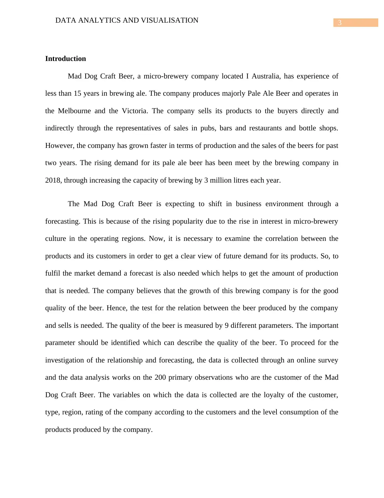
Introduction
Mad Dog Craft Beer, a micro-brewery company located I Australia, has experience of
less than 15 years in brewing ale. The company produces majorly Pale Ale Beer and operates in
the Melbourne and the Victoria. The company sells its products to the buyers directly and
indirectly through the representatives of sales in pubs, bars and restaurants and bottle shops.
However, the company has grown faster in terms of production and the sales of the beers for past
two years. The rising demand for its pale ale beer has been meet by the brewing company in
2018, through increasing the capacity of brewing by 3 million litres each year.
The Mad Dog Craft Beer is expecting to shift in business environment through a
forecasting. This is because of the rising popularity due to the rise in interest in micro-brewery
culture in the operating regions. Now, it is necessary to examine the correlation between the
products and its customers in order to get a clear view of future demand for its products. So, to
fulfil the market demand a forecast is also needed which helps to get the amount of production
that is needed. The company believes that the growth of this brewing company is for the good
quality of the beer. Hence, the test for the relation between the beer produced by the company
and sells is needed. The quality of the beer is measured by 9 different parameters. The important
parameter should be identified which can describe the quality of the beer. To proceed for the
investigation of the relationship and forecasting, the data is collected through an online survey
and the data analysis works on the 200 primary observations who are the customer of the Mad
Dog Craft Beer. The variables on which the data is collected are the loyalty of the customer,
type, region, rating of the company according to the customers and the level consumption of the
products produced by the company.
Paraphrase This Document
Need a fresh take? Get an instant paraphrase of this document with our AI Paraphraser
4DATA ANALYTICS AND VISUALISATION
Description
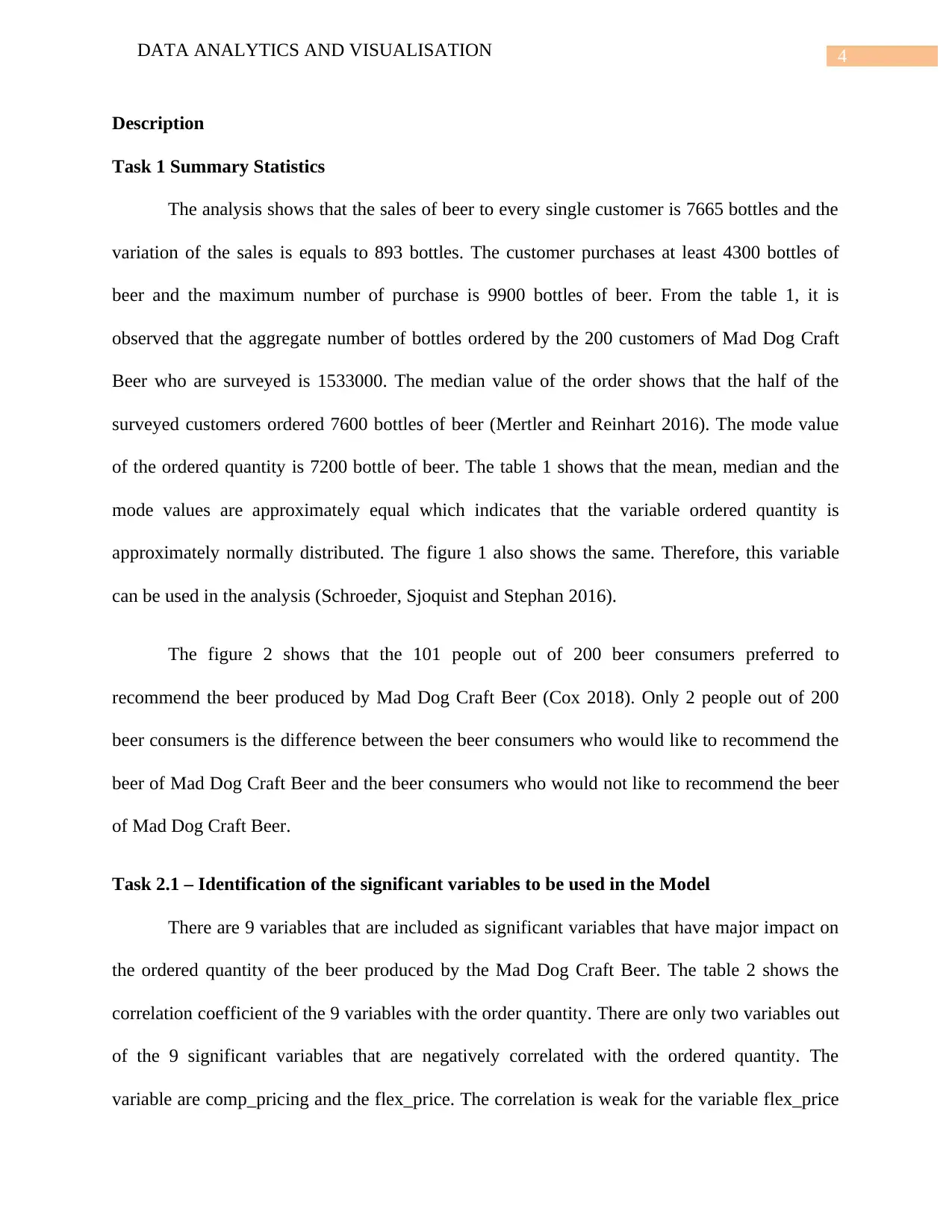
Task 1 Summary Statistics
The analysis shows that the sales of beer to every single customer is 7665 bottles and the
variation of the sales is equals to 893 bottles. The customer purchases at least 4300 bottles of
beer and the maximum number of purchase is 9900 bottles of beer. From the table 1, it is
observed that the aggregate number of bottles ordered by the 200 customers of Mad Dog Craft
Beer who are surveyed is 1533000. The median value of the order shows that the half of the
surveyed customers ordered 7600 bottles of beer (Mertler and Reinhart 2016). The mode value
of the ordered quantity is 7200 bottle of beer. The table 1 shows that the mean, median and the
mode values are approximately equal which indicates that the variable ordered quantity is
approximately normally distributed. The figure 1 also shows the same. Therefore, this variable
can be used in the analysis (Schroeder, Sjoquist and Stephan 2016).
The figure 2 shows that the 101 people out of 200 beer consumers preferred to
recommend the beer produced by Mad Dog Craft Beer (Cox 2018). Only 2 people out of 200
beer consumers is the difference between the beer consumers who would like to recommend the
beer of Mad Dog Craft Beer and the beer consumers who would not like to recommend the beer
of Mad Dog Craft Beer.
Task 2.1 – Identification of the significant variables to be used in the Model
There are 9 variables that are included as significant variables that have major impact on
the ordered quantity of the beer produced by the Mad Dog Craft Beer. The table 2 shows the
correlation coefficient of the 9 variables with the order quantity. There are only two variables out
of the 9 significant variables that are negatively correlated with the ordered quantity. The
variable are comp_pricing and the flex_price. The correlation is weak for the variable flex_price
Description
Task 1 Summary Statistics
The analysis shows that the sales of beer to every single customer is 7665 bottles and the
variation of the sales is equals to 893 bottles. The customer purchases at least 4300 bottles of
beer and the maximum number of purchase is 9900 bottles of beer. From the table 1, it is
observed that the aggregate number of bottles ordered by the 200 customers of Mad Dog Craft
Beer who are surveyed is 1533000. The median value of the order shows that the half of the
surveyed customers ordered 7600 bottles of beer (Mertler and Reinhart 2016). The mode value
of the ordered quantity is 7200 bottle of beer. The table 1 shows that the mean, median and the
mode values are approximately equal which indicates that the variable ordered quantity is
approximately normally distributed. The figure 1 also shows the same. Therefore, this variable
can be used in the analysis (Schroeder, Sjoquist and Stephan 2016).
The figure 2 shows that the 101 people out of 200 beer consumers preferred to
recommend the beer produced by Mad Dog Craft Beer (Cox 2018). Only 2 people out of 200
beer consumers is the difference between the beer consumers who would like to recommend the
beer of Mad Dog Craft Beer and the beer consumers who would not like to recommend the beer
of Mad Dog Craft Beer.
Task 2.1 – Identification of the significant variables to be used in the Model
There are 9 variables that are included as significant variables that have major impact on
the ordered quantity of the beer produced by the Mad Dog Craft Beer. The table 2 shows the
correlation coefficient of the 9 variables with the order quantity. There are only two variables out
of the 9 significant variables that are negatively correlated with the ordered quantity. The
variable are comp_pricing and the flex_price. The correlation is weak for the variable flex_price
5DATA ANALYTICS AND VISUALISATION
as the correlation coefficient is very close to zero (Meyers, Gamst and Guarin 2016). The
comp_pricing has a negative impact on the dependent variable that is ordered quantity which is
negligible. Thus the two variable with negative correlation are omitted for the further steps of
analysis. The remaining seven variables that are able to impact the dependent variable positively.
The strongest correlation is found between the shipping_cost and the order quantity. The
correlation coefficient for the shipping_cost is 0.504413. Other than this variable, there are
quality, shipping_speed and brand_image with the correlation coefficient 0.433372, 0.425082
and 0.338005 respectively that shows moderate correlation with the dependent variable (Gordon
2015). The variables that shows the weak correlation with the dependent variable are
sm_prsence, advert and order_fulfillment as the correlation coefficient are 0.235189, 0.237038
and 0.314591 respectively.
Task 2.2 – Model Building
2.2a - First Model
The analysis includes the seven variables to use them in the predictive analysis and the
variables are Product Quality, Social Media Presence, Advertising, Brand Image, Order &
Billing, Shipping Speed and Shipping Cost. In the previous section, it is seen that these seven
variables show the positive correlation and can influence the order quantity positively.
The first step to build the model in order to predict the dependent variable, the linear
multiple regression is considered to be used.
The model for the prediction of the order quantity can be represented as below:
Order Quanity=3.033+ 0.277∗Quality−0.156∗SM Presence−0. 018∗Advert +0. .322∗Brand Image−0.149
⊘ This is a preview!⊘
Do you want full access?
Subscribe today to unlock all pages.
Trusted by 1+ million students worldwide
6DATA ANALYTICS AND VISUALISATION
The regression result gives the coefficients of the variables that are used to form the above
equation. The regression result is presented in the table 3. The table also reveals that the
coefficient of the variables Social Media Presence, Advertising Order & Billing and Shipping
Speed are not significant as the p-value are greater than 0.05. The p-value for the intercept,
quality, brand image and shipping cost is 0.0, 0. 0, 0.0 and 0.01 which indicates that there is
enough evidence that the coefficient are significant at 5% significance level. Now, it can be
concluded that other variables reaming constant, the ordered quantity can be influenced by the
quality, brand image and shipping cost by the factor 0.2777, 0.322 and 0.257. The variables that
are not significant at a standard significance level have the negative impact on the order quantity.
For example, one unit of increase in advertising reduces the order quantity by 0.018 amount as
the coefficient of the variable is -0.018. Same thing happens for the Social Media Presence and
Order & Billing. The remaining variable that have a no significant impact on the ordered
quantity is shipping speed which has the coefficient 0.174. Therefore, the four insignificant
variables (SM presence, advertisement, order fulfilment and shipping speed are dropped to
predict appropriately in further analysis of order quantity (Chatterjee and Hadi 2015).
Moreover, the adjusted R2 is equal to 0.454 that indicates the prediction of the ordered
quantity is 45.4% by the seven variables that are included in the analysis (Nakagawa, S., Johnson
and Schielzeth 2017). The independent variables are able to influence the dependent variable
significantly and the f-stat is F (7, 192) = 24.604 (Fox 2015).
2.2b - Second model
The second model omits the insignificant variables of the previous regression (Table 3:
regression result of the previous model shows the insignificant variables) in order to get the
better result by creating a better model with the significant variables only. The second model
Paraphrase This Document
Need a fresh take? Get an instant paraphrase of this document with our AI Paraphraser
7DATA ANALYTICS AND VISUALISATION
includes the significant variables that are Quality, Brand Image and Shipping Cost. The omitted
variable are SM Presence, Advertisement, Order fulfilment and Shipping Speed with p-value less
than 0.05. The second model is presented below:
Order Quantity=2.924+ 0.268∗Quality +0.220∗Brand Image +0.273∗Shipping Cost
The table 4 shows that for the above linear multiple regression model adjusted R2 is found to
be 0.449. This indicates that prediction of the ordered quantity of Mad Dog Craft Beer is 44.9%
after excluding the insignificant variables and by the fours variables that are included in the
analysis (Chatfield 2018). The independent variables are able to influence the dependent variable
significantly as the f-stat is F (3, 192) = 55.003. The three variables along with the intercept term
is statistically significant at 5% level as the p-value for the coefficients of the variables are less
than 0.05. The coefficient of the quality is 0.268 with 0.00 which indicates that one unit increase
in the quantity will raise the order quantity of Mad Dog Craft Beer by 0.268 unit. The coefficient
of the brand image is 0.220 with p-value 0.00 which indicates that one unit increase in the brand
image will raise the order quantity of Mad Dog Craft Beer by 0.220 unit. The coefficient of the
shipping cost is 0.273 with p-value 0.00 which indicates that one unit increase in the shipping
cost will raise the order quantity of Mad Dog Craft Beer by 0.273 unit.
Finally, it can be said that the Mad Dog Craft Beer should consider only the views of
customers on the variables Quality, Brand Image and Shipping Cost. Thus, the prediction will be
robust, consistent and efficient.
Task 2.3 – Interaction Effect
To analyse the interaction effect of the variable Brand Image on the relation between
Quality and Order Quantity of Mad Dog Craft Beer, an interaction variable is introduced in the
8DATA ANALYTICS AND VISUALISATION
model. The interaction variable is nothing but the product of customer responses of quality and
brand image (Schumacker 2017). Now, these three variables Quality, Brand image and
Interaction term are the independent variables in the model that analyse the interaction effect.
Order quantity is the dependent variable as in the previous model. Multiple linear regression is
used to study the interaction effect as the model follows all the assumptions of linear regression
(Hox, Moerbeek and Van de Schoot 2017). The interaction effect is analysed by the following
model:
Order Quanity=0.5011+ 0.6911∗Quality +0.8643∗Brand Image−0.0686∗Quality∗Brand Image
From the table 5, it is found that the intercept term is 0.5011 with p-value 0.7447 that means
the intercept term is insignificant. The coefficient of the quality is 0.6911 with p-value 0.0003
which indicates that one unite increase in the quality will significantly raise the order quantity of
Mad Dog Craft Beer by 0.6911 unit at 5% significance level. The coefficient of the brand image
is 0.8643 with p-value 0.0013 which indicates that one unit increase in the brand image will
significantly raise the order quantity of Mad Dog Craft Beer by 0.8643 unit at 5% significance
level. The coefficient of the interaction term is -0.0686 with p-value 0.0387 which indicates that
one unit increase in the interaction term will significantly reduce the order quantity of Mad Dog
Craft Beer by 0.0686 unit at 5% significance level (Austin and Juan Merlo 2017).
⊘ This is a preview!⊘
Do you want full access?
Subscribe today to unlock all pages.
Trusted by 1+ million students worldwide
9DATA ANALYTICS AND VISUALISATION
Task 3
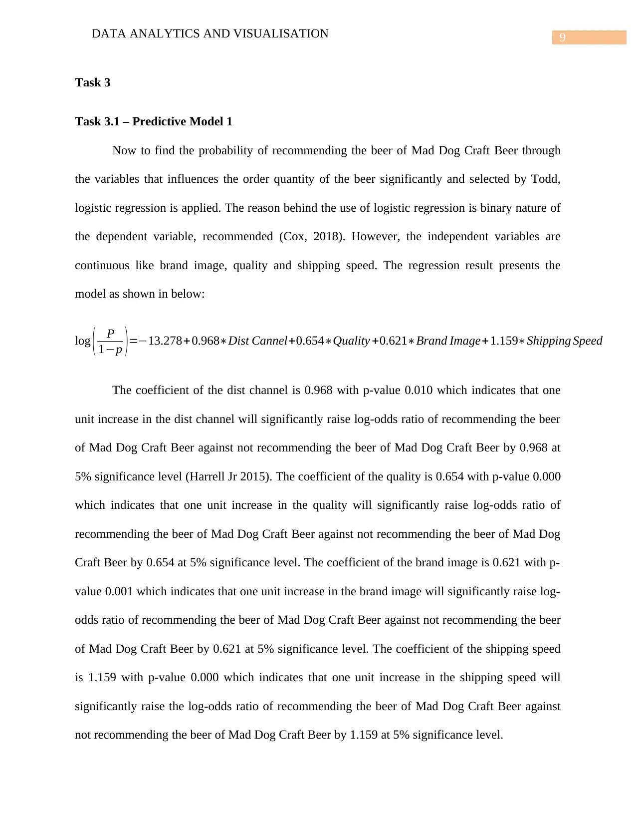
Task 3.1 – Predictive Model 1
Now to find the probability of recommending the beer of Mad Dog Craft Beer through
the variables that influences the order quantity of the beer significantly and selected by Todd,
logistic regression is applied. The reason behind the use of logistic regression is binary nature of
the dependent variable, recommended (Cox, 2018). However, the independent variables are
continuous like brand image, quality and shipping speed. The regression result presents the
model as shown in below:
log ( P
1−p )=−13.278+ 0.968∗Dist Cannel+0.654∗Quality +0.621∗Brand Image+ 1.159∗Shipping Speed
The coefficient of the dist channel is 0.968 with p-value 0.010 which indicates that one
unit increase in the dist channel will significantly raise log-odds ratio of recommending the beer
of Mad Dog Craft Beer against not recommending the beer of Mad Dog Craft Beer by 0.968 at
5% significance level (Harrell Jr 2015). The coefficient of the quality is 0.654 with p-value 0.000
which indicates that one unit increase in the quality will significantly raise log-odds ratio of
recommending the beer of Mad Dog Craft Beer against not recommending the beer of Mad Dog
Craft Beer by 0.654 at 5% significance level. The coefficient of the brand image is 0.621 with p-
value 0.001 which indicates that one unit increase in the brand image will significantly raise log-
odds ratio of recommending the beer of Mad Dog Craft Beer against not recommending the beer
of Mad Dog Craft Beer by 0.621 at 5% significance level. The coefficient of the shipping speed
is 1.159 with p-value 0.000 which indicates that one unit increase in the shipping speed will
significantly raise the log-odds ratio of recommending the beer of Mad Dog Craft Beer against
not recommending the beer of Mad Dog Craft Beer by 1.159 at 5% significance level.
Task 3
Task 3.1 – Predictive Model 1
Now to find the probability of recommending the beer of Mad Dog Craft Beer through
the variables that influences the order quantity of the beer significantly and selected by Todd,
logistic regression is applied. The reason behind the use of logistic regression is binary nature of
the dependent variable, recommended (Cox, 2018). However, the independent variables are
continuous like brand image, quality and shipping speed. The regression result presents the
model as shown in below:
log ( P
1−p )=−13.278+ 0.968∗Dist Cannel+0.654∗Quality +0.621∗Brand Image+ 1.159∗Shipping Speed
The coefficient of the dist channel is 0.968 with p-value 0.010 which indicates that one
unit increase in the dist channel will significantly raise log-odds ratio of recommending the beer
of Mad Dog Craft Beer against not recommending the beer of Mad Dog Craft Beer by 0.968 at
5% significance level (Harrell Jr 2015). The coefficient of the quality is 0.654 with p-value 0.000
which indicates that one unit increase in the quality will significantly raise log-odds ratio of
recommending the beer of Mad Dog Craft Beer against not recommending the beer of Mad Dog
Craft Beer by 0.654 at 5% significance level. The coefficient of the brand image is 0.621 with p-
value 0.001 which indicates that one unit increase in the brand image will significantly raise log-
odds ratio of recommending the beer of Mad Dog Craft Beer against not recommending the beer
of Mad Dog Craft Beer by 0.621 at 5% significance level. The coefficient of the shipping speed
is 1.159 with p-value 0.000 which indicates that one unit increase in the shipping speed will
significantly raise the log-odds ratio of recommending the beer of Mad Dog Craft Beer against
not recommending the beer of Mad Dog Craft Beer by 1.159 at 5% significance level.
Paraphrase This Document
Need a fresh take? Get an instant paraphrase of this document with our AI Paraphraser
10DATA ANALYTICS AND VISUALISATION
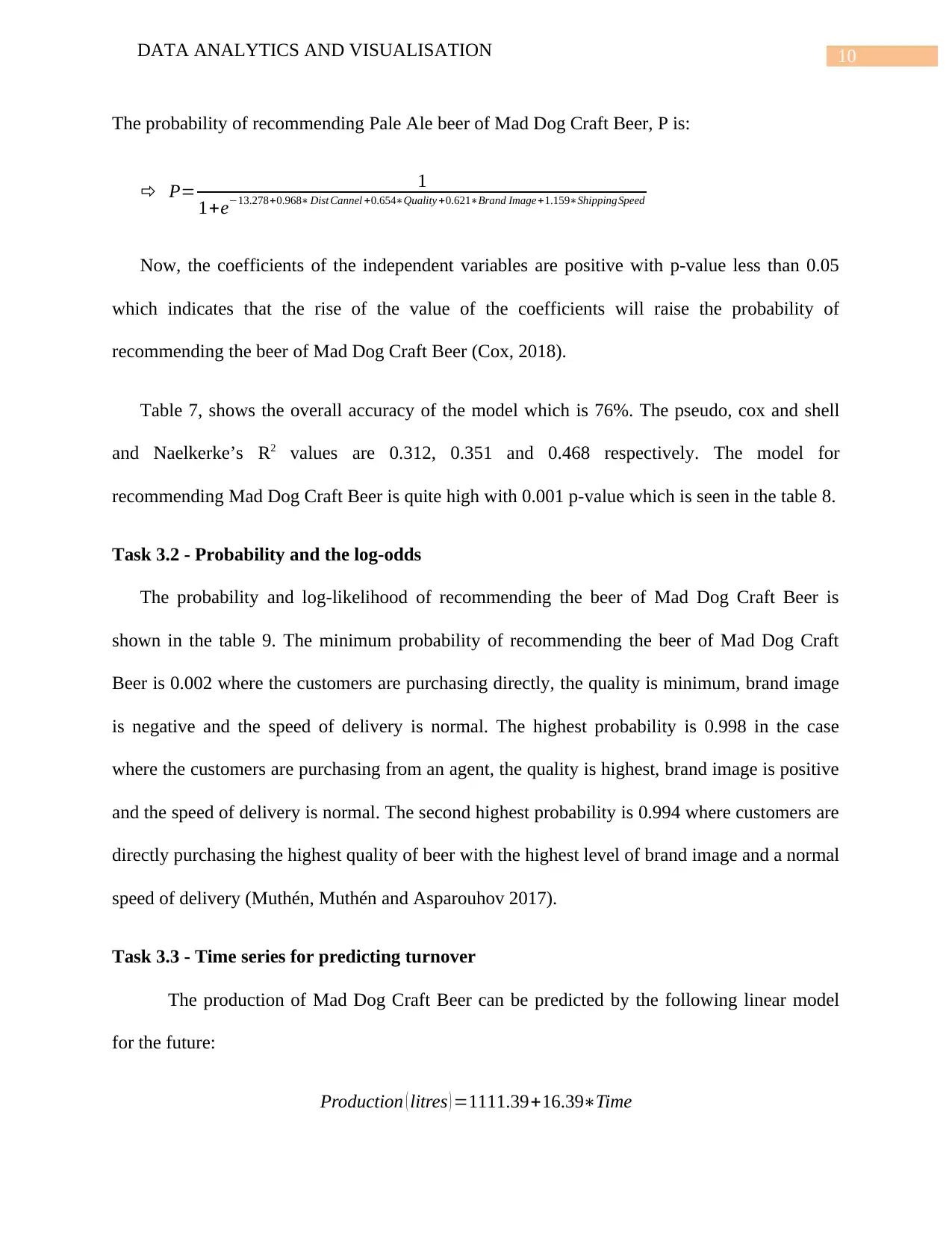
The probability of recommending Pale Ale beer of Mad Dog Craft Beer, P is:
P= 1
1+e−13.278+0.968∗ Dist Cannel +0.654∗Quality +0.621∗Brand Image +1.159∗ShippingSpeed
Now, the coefficients of the independent variables are positive with p-value less than 0.05
which indicates that the rise of the value of the coefficients will raise the probability of
recommending the beer of Mad Dog Craft Beer (Cox, 2018).
Table 7, shows the overall accuracy of the model which is 76%. The pseudo, cox and shell
and Naelkerke’s R2 values are 0.312, 0.351 and 0.468 respectively. The model for
recommending Mad Dog Craft Beer is quite high with 0.001 p-value which is seen in the table 8.
Task 3.2 - Probability and the log-odds
The probability and log-likelihood of recommending the beer of Mad Dog Craft Beer is
shown in the table 9. The minimum probability of recommending the beer of Mad Dog Craft
Beer is 0.002 where the customers are purchasing directly, the quality is minimum, brand image
is negative and the speed of delivery is normal. The highest probability is 0.998 in the case
where the customers are purchasing from an agent, the quality is highest, brand image is positive
and the speed of delivery is normal. The second highest probability is 0.994 where customers are
directly purchasing the highest quality of beer with the highest level of brand image and a normal
speed of delivery (Muthén, Muthén and Asparouhov 2017).
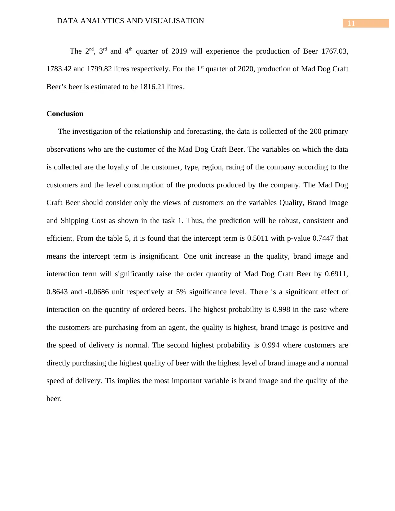
Task 3.3 - Time series for predicting turnover
The production of Mad Dog Craft Beer can be predicted by the following linear model
for the future:
Production ( litres ) =1111.39+16.39∗Time
The probability of recommending Pale Ale beer of Mad Dog Craft Beer, P is:
P= 1
1+e−13.278+0.968∗ Dist Cannel +0.654∗Quality +0.621∗Brand Image +1.159∗ShippingSpeed
Now, the coefficients of the independent variables are positive with p-value less than 0.05
which indicates that the rise of the value of the coefficients will raise the probability of
recommending the beer of Mad Dog Craft Beer (Cox, 2018).
Table 7, shows the overall accuracy of the model which is 76%. The pseudo, cox and shell
and Naelkerke’s R2 values are 0.312, 0.351 and 0.468 respectively. The model for
recommending Mad Dog Craft Beer is quite high with 0.001 p-value which is seen in the table 8.
Task 3.2 - Probability and the log-odds
The probability and log-likelihood of recommending the beer of Mad Dog Craft Beer is
shown in the table 9. The minimum probability of recommending the beer of Mad Dog Craft
Beer is 0.002 where the customers are purchasing directly, the quality is minimum, brand image
is negative and the speed of delivery is normal. The highest probability is 0.998 in the case
where the customers are purchasing from an agent, the quality is highest, brand image is positive
and the speed of delivery is normal. The second highest probability is 0.994 where customers are
directly purchasing the highest quality of beer with the highest level of brand image and a normal
speed of delivery (Muthén, Muthén and Asparouhov 2017).
Task 3.3 - Time series for predicting turnover
The production of Mad Dog Craft Beer can be predicted by the following linear model
for the future:
Production ( litres ) =1111.39+16.39∗Time
11DATA ANALYTICS AND VISUALISATION
The 2nd, 3rd and 4th quarter of 2019 will experience the production of Beer 1767.03,
1783.42 and 1799.82 litres respectively. For the 1st quarter of 2020, production of Mad Dog Craft
Beer’s beer is estimated to be 1816.21 litres.
Conclusion
The investigation of the relationship and forecasting, the data is collected of the 200 primary
observations who are the customer of the Mad Dog Craft Beer. The variables on which the data
is collected are the loyalty of the customer, type, region, rating of the company according to the
customers and the level consumption of the products produced by the company. The Mad Dog
Craft Beer should consider only the views of customers on the variables Quality, Brand Image
and Shipping Cost as shown in the task 1. Thus, the prediction will be robust, consistent and
efficient. From the table 5, it is found that the intercept term is 0.5011 with p-value 0.7447 that
means the intercept term is insignificant. One unit increase in the quality, brand image and
interaction term will significantly raise the order quantity of Mad Dog Craft Beer by 0.6911,
0.8643 and -0.0686 unit respectively at 5% significance level. There is a significant effect of
interaction on the quantity of ordered beers. The highest probability is 0.998 in the case where
the customers are purchasing from an agent, the quality is highest, brand image is positive and
the speed of delivery is normal. The second highest probability is 0.994 where customers are
directly purchasing the highest quality of beer with the highest level of brand image and a normal
speed of delivery. Tis implies the most important variable is brand image and the quality of the
beer.
⊘ This is a preview!⊘
Do you want full access?
Subscribe today to unlock all pages.
Trusted by 1+ million students worldwide
1 out of 20
Related Documents


Your All-in-One AI-Powered Toolkit for Academic Success.
+13062052269
info@desklib.com
Available 24*7 on WhatsApp / Email
![[object Object]](/_next/static/media/star-bottom.7253800d.svg)
Unlock your academic potential
Copyright © 2020–2026 A2Z Services. All Rights Reserved. Developed and managed by ZUCOL.