BUS105 Computing Assignment: Dataset and Variable Analysis

This assignment solution for BUS105 focuses on data analysis techniques, covering datasets, variables, and their comparison methods. The document defines datasets, categorical and numerical variables, and methods like scatterplots and pivot tables. It includes examples analyzing the relationship between distance travelled and selling price, using z-scores and confidence intervals. The assignment explores comparing proportions, analyzing sample means, and summarizing data using back-to-back histograms and confidence intervals, demonstrating practical applications of data analysis in various scenarios. The solution provides detailed steps, calculations, and interpretations of the results, including pivot tables, graphs, and statistical analyses to compare different variables and draw conclusions.

Running Head: BUS105 COMPUTING ASSIGNMENT
BUS105
Computing Assignment
Name of the Student
Student Number
Allocated Sample: 116

1BUS105 COMPUTING ASSIGNMENT
Executive Summary
This study is mainly about the techniques for the comparison of different types of variables in a
dataset. The first section of the study involves the definitions of datasets, variables, and types of
variables and how to compare different types of variables. Illustrations on comparison of
different types of variables are described in the following sections.

2BUS105 COMPUTING ASSIGNMENT
Table of Contents
Section 1..........................................................................................................................................3
Section 2..........................................................................................................................................5
Section 3..........................................................................................................................................6
Section 4..........................................................................................................................................8
Section 5........................................................................................................................................10
Section 6........................................................................................................................................11

3BUS105 COMPUTING ASSIGNMENT
Section 1
A dataset is usually a collection of data. These data can be of items that are discrete and
related. These can be assessed separately or together with other variables. Thus, data arranged
properly and in the form of tables is known as a dataset. For example, there can be a collection of
names, contact information, salaries, sales figures etc. in a file. This whole collection is known as
a dataset and all these individual entities can be dealt with separately and also with relation of
other variables or even considering all the variables at the same time.
A variable is termed as a value which changes from time to time. The changes are
dependent on the conditions and the situations. Variables usually contain some values which
represent certain characteristics. Variables can be of two types, Categorical and Numerical.
Categorical variables are qualitative variables and they represent some categories whereas
numerical variables contain numeric values. Numerical variables can be discrete and continuous
as well. Example of a categorical variable is gender of a person which can be either male or
female. Example of a discrete numeric variable is the number of phone calls received by a person
in a day where the values are distinct and countable. An example of a continuous random
variable is the income of people.
There are certain ways to summarize datasets on the basis of the type of variables that are
involved in the dataset. The relationship between two variables can be expressed in the following
ways:
 If both the variables are quantitative or numerical, then the relationship between the two
variables can be expressed diagrammatically with the help of a scatterplot.

4BUS105 COMPUTING ASSIGNMENT
 If both the variables are categorical, then the relationship between the two variables can
be expressed by comparing the proportions of the two variables.
 If there is one categorical and one numeric variable, then the relationship between the
two variables can be expressed in the simplest manner by comparing the means of the
different categories.
There are certain features in computing softwares that can analyze and summarize data in
a very simple and faster manner. Some advanced features are there in Microsoft Excel such as
pivot tables and filtering with the help of which data can be summarized very easily. Thus, to
reduce the labour and time of computing, computer softwares are used to summarize data.

5BUS105 COMPUTING ASSIGNMENT
Section 2
(a) The scatterplot of distance travelled and selling price is given below:
15000 20000 25000 30000 35000 40000 45000 50000 55000
0
2000
4000
6000
8000
10000
12000
14000
16000
18000
20000
f(x) = − 0.249880702257711 x + 22147.6745701038
Scatterplot
Distance Travelled
Selling Price
It can be seen from the scatterplot that distance travelled and selling price of the cars are
negatively related. That is, if the distance travelled by the car increases, the selling price of the
car decreases. The line that best fits the model is given by y = -0.2499x + 22148, where y is the
selling price of the car and x is the distance travelled.
(b) An estimate of the selling price of the car that has travelled 30,000 km is
Predicted selling price = (-0.2499 * 30000) + 22148 = $14651.
(c) Population mean = 14,000
Population standard deviation = 392.
Therefore, z-score = (14651 – 14000)/392 = 1.66
(d) P (Z < 1.66) = 0.9515, obtained from wolphramalpha.com
(e) Comparing sample 116 to the 10,000 samples, the expected rank to which the sample will
be close to is:

6BUS105 COMPUTING ASSIGNMENT
Expected Rank = P (Z < z-score) * 10000 = 0.9515 * 10,000 = 9515
Section 3
(a) The required pivot tables are given below:
which sample ? 116
Count of Do they like it ? (y=yes, n=no) Column Labels
Row Labels n y
Grand
Total
A 11 83 94
B 19 88 107
Grand Total 30 171 201
which sample ? 116
Count of Do they like it ? (y=yes, n=no) Column Labels
Row Labels n y
Grand
Total
A 11.70%
88.30
% 100.00%
B 17.76%
82.24
% 100.00%
Grand Total 14.93%
85.07
% 100.00%
(b) Graph comparing the proportions found in part a is given below:

7BUS105 COMPUTING ASSIGNMENT
(c) From the observations in parts a and b it can be seen that more people like version A than
version B.
(d) i) Estimated difference in proportions for sample 116 = 0.8830 – 0.8224 = 0.0606
ii) Average of 1000 sample estimates = 0.1
Standard deviation of 1000 sample estimates = 0.0505.
Therefore, z-score for sample 116 = (0.0606-0.1) / 0.0505 = -0.78
iii) P (Z < -0.78) = 0.2177, obtained from wolphramalpha.com
iv) Expected rank for sample 116 is given by:
Expected Rank = P (Z < z-score) * 1000 = 0.2177 * 1000 = 217
(e) i) H0: p1 = p2
H1: p1 ≠ p2
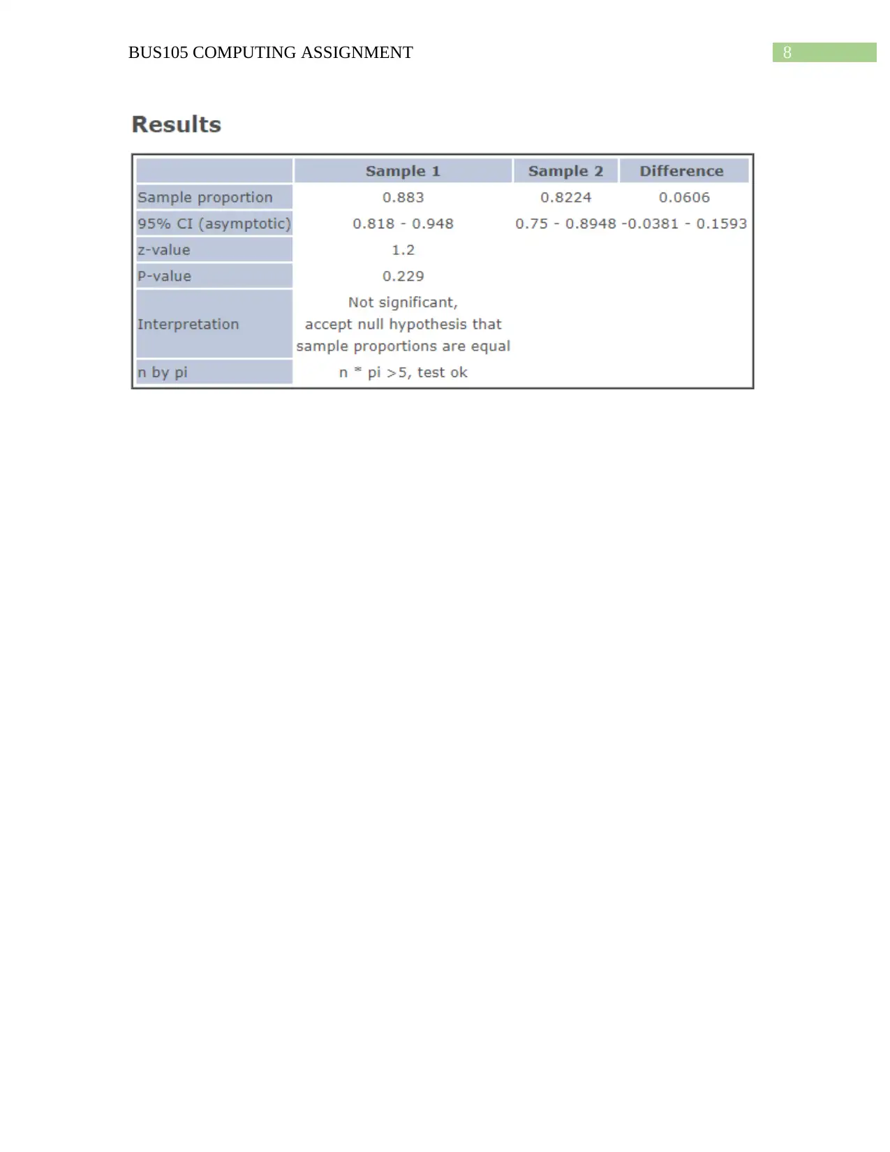
ii) The p-value has been obtained as 0.229
iii) H0 is accepted.
iv) It can be said that the sample proportions are equal.

8BUS105 COMPUTING ASSIGNMENT

9BUS105 COMPUTING ASSIGNMENT
Section 4
(a) Pivot table showing the appropriate summary statistics for sample 116 is given below:
which
sample? 116
Row Labels
Count of which machine?
(A or B)
Average of $ Casino profit
from bet
StdDev of $ Casino profit
from bet2
A 95 0.473684211 4.368265894
B 105 0.142857143 1.361761949
Grand
Total 200 0.3 3.163866345
(b) The profit from bet from machine A at a Casino on an average is $0.47 with a deviation
of $4.37 which is very high. Thus the profits from machine A are not always close to the
average profit.
The profit from bet from machine B at a Casino on an average is $0.14 with a deviation
of $1.36 which is not very high. Thus the profits from machine B are not mostly close to
the average profit.
(c) i) the estimated difference between the sample means for sample 116 = (0.47 – 0.14) =
0.33
ii) For the 2000 sample estimates, average = 0.4
Standard deviation = 0.46
Therefore, z-score for sample 116 = (0.33 – 0.4)/0.46 = -0.15
iii) P (Z < -0.15) = 0.5596, obtained from wolphramalpha.com
iv) Expected rank for sample 116 is given by:
Expected Rank = P (Z < z-score) * 1000 = 0.5596 * 1000 = 559
(d) i) H0: μ1 = μ2

10BUS105 COMPUTING ASSIGNMENT
H1: μ1 ≠μ2
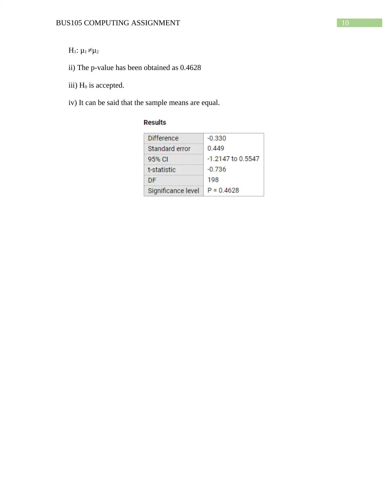
ii) The p-value has been obtained as 0.4628
iii) H0 is accepted.
iv) It can be said that the sample means are equal.

11BUS105 COMPUTING ASSIGNMENT
Section 5
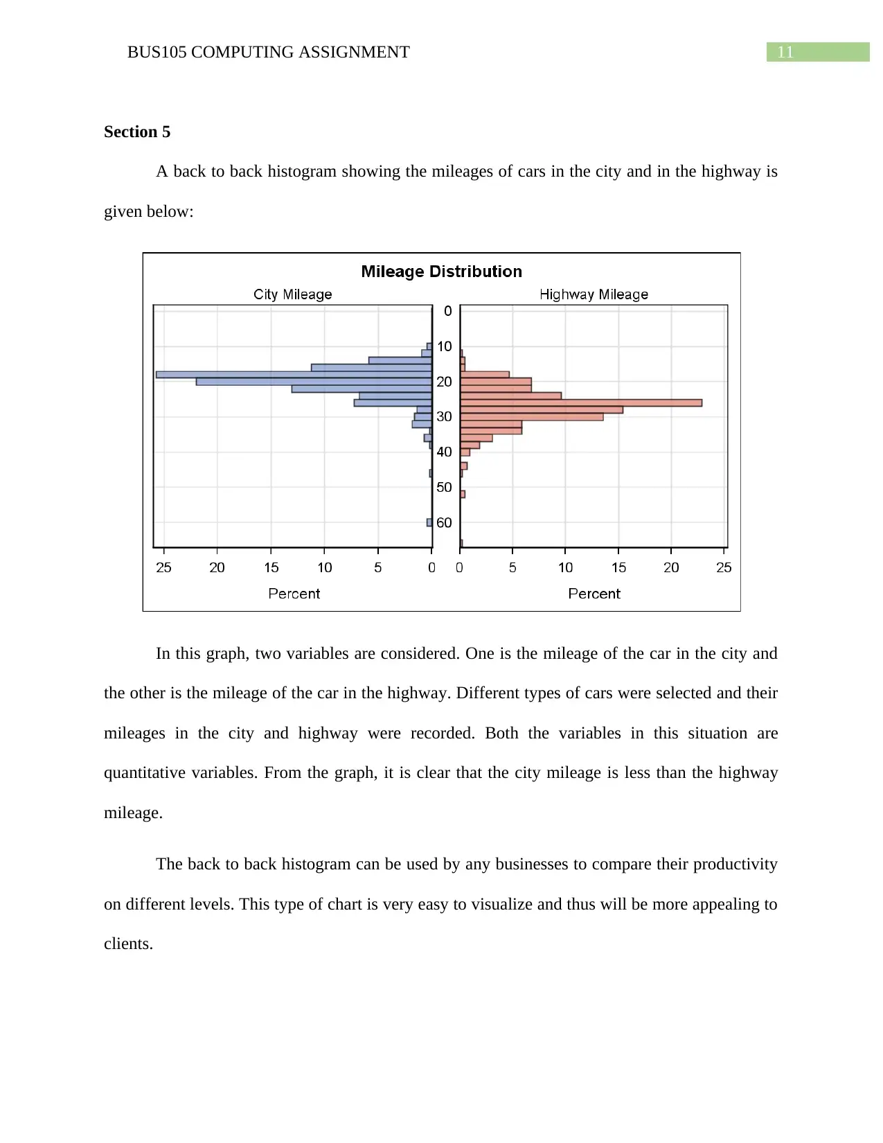
A back to back histogram showing the mileages of cars in the city and in the highway is
given below:
In this graph, two variables are considered. One is the mileage of the car in the city and
the other is the mileage of the car in the highway. Different types of cars were selected and their
mileages in the city and highway were recorded. Both the variables in this situation are
quantitative variables. From the graph, it is clear that the city mileage is less than the highway
mileage.
The back to back histogram can be used by any businesses to compare their productivity
on different levels. This type of chart is very easy to visualize and thus will be more appealing to
clients.

12BUS105 COMPUTING ASSIGNMENT
Section 6
(a) Table showing summary of the given data for sample 116 is given below
Row
Labels
Count of do you support proposed
change?
Proportion of do you support proposed
change?2
no 91 0.471502591
yes 102 0.528497409
Grand
Total 193 1
(b) For sample 116, sample size = 193.
Support for the proposed change = 102
Therefore, proportion of success = (102/193) = 0.5285
(c) i) For the 1000 estimates,
Average = 0.6
Standard deviation = 0.0357.
Therefore, z-score for sample 116 is = (0.5285 – 0.6)/0.0357 = -2.00
ii) P (Z < -2.00) = 0.0228, obtained from wolphramalpha.com
iii) If we compare the sample 116 to the 1000 other estimates, then we estimate the rank
to be 0.0228 * 1000 = 22
(d) A 95% confidence interval for the proportion of people that support the change is given
by (0.456, 0.601)