DC Motor Control System Design and MATLAB Analysis
VerifiedAdded on 2022/08/27
|22
|3852
|13
Project
AI Summary
This assignment presents a comprehensive analysis and control system design for a DC motor using MATLAB. Part 1 focuses on data processing and analysis, calculating yaw angle, distance traveled, and accelerations for a rally stage dataset. Part 2 delves into the DC motor's step response using a transfer function, providing MATLAB code and a stability analysis. The assignment further explores the design and comparison of P, PI, and PID controllers for the DC motor, evaluating parameters such as rise time, settling time, steady-state error, and overshoot. The solution includes MATLAB code for each controller type and a detailed discussion of the controller design steps and their impact on system performance. The appendices contain the MATLAB code used for data processing, analysis and controller implementation.
PART: 1
Data processing and analysis
1. Calculate the yaw angle, distance travelled, longitudinal, lateral acceleration,
path curvature with distance travelled and the full lap in the rally stage data set.
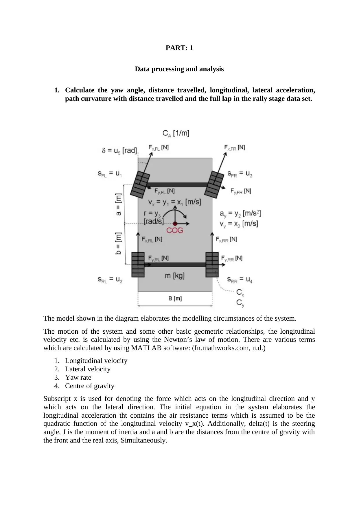
The model shown in the diagram elaborates the modelling circumstances of the system.
The motion of the system and some other basic geometric relationships, the longitudinal
velocity etc. is calculated by using the Newton’s law of motion. There are various terms
which are calculated by using MATLAB software: (In.mathworks.com, n.d.)
1. Longitudinal velocity
2. Lateral velocity
3. Yaw rate
4. Centre of gravity
Subscript x is used for denoting the force which acts on the longitudinal direction and y
which acts on the lateral direction. The initial equation in the system elaborates the
longitudinal acceleration tht contains the air resistance terms which is assumed to be the
quadratic function of the longitudinal velocity v_x(t). Additionally, delta(t) is the steering
angle, J is the moment of inertia and a and b are the distances from the centre of gravity with
the front and the real axis, Simultaneously.
Data processing and analysis
1. Calculate the yaw angle, distance travelled, longitudinal, lateral acceleration,
path curvature with distance travelled and the full lap in the rally stage data set.
The model shown in the diagram elaborates the modelling circumstances of the system.
The motion of the system and some other basic geometric relationships, the longitudinal
velocity etc. is calculated by using the Newton’s law of motion. There are various terms
which are calculated by using MATLAB software: (In.mathworks.com, n.d.)
1. Longitudinal velocity
2. Lateral velocity
3. Yaw rate
4. Centre of gravity
Subscript x is used for denoting the force which acts on the longitudinal direction and y
which acts on the lateral direction. The initial equation in the system elaborates the
longitudinal acceleration tht contains the air resistance terms which is assumed to be the
quadratic function of the longitudinal velocity v_x(t). Additionally, delta(t) is the steering
angle, J is the moment of inertia and a and b are the distances from the centre of gravity with
the front and the real axis, Simultaneously.
Paraphrase This Document
Need a fresh take? Get an instant paraphrase of this document with our AI Paraphraser
In these equations Cx and Cy can be termed as the longitudinal and the lateral tire stiffness.
Here it is being assumed that these stiffness parameters are similar for all 4 tires.
PART: 2
1. In MATLAB, plot the step response of the provided DC motor using the transfer
function. Please provide MATLAB code or a Simulink model.
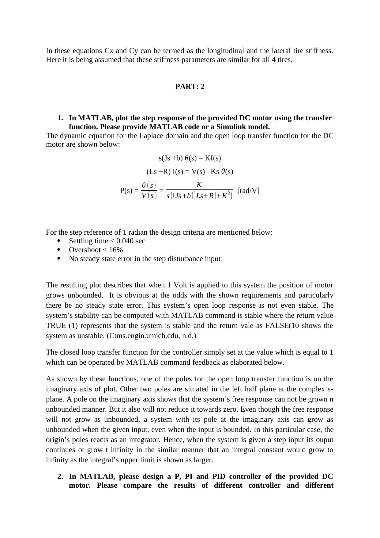
The dynamic equation for the Laplace domain and the open loop transfer function for the DC
motor are shown below:
s(Js +b) θ(s) = KI(s)
(Ls +R) I(s) = V(s) –Ks θ(s)
P(s) = θ (s)
V (s ) = K
s ( ( Js +b ) ( Ls+ R ) + K2) [rad/V]
For the step reference of 1 radian the design criteria are mentioned below:
Settling time < 0.040 sec
Overshoot < 16%
No steady state error in the step disturbance input
The resulting plot describes that when 1 Volt is applied to this system the position of motor
grows unbounded. It is obvious at the odds with the shown requirements and particularly
there be no steady state error. This system’s open loop response is not even stable. The
system’s stability can be computed with MATLAB command is stable where the return value
TRUE (1) represents that the system is stable and the return vale as FALSE(10 shows the
system as unstable. (Ctms.engin.umich.edu, n.d.)
The closed loop transfer function for the controller simply set at the value which is equal to 1
which can be operated by MATLAB command feedback as elaborated below.
As shown by these functions, one of the poles for the open loop transfer function is on the
imaginary axis of plot. Other two poles are situated in the left half plane at the complex s-
plane. A pole on the imaginary axis shows that the system’s free response can not be grown n
unbounded manner. But it also will not reduce it towards zero. Even though the free response
will not grow as unbounded, a system with its pole at the imaginary axis can grow as
unbounded when the given input, even when the input is bounded. In this particular case, the
origin’s poles reacts as an integrator. Hence, when the system is given a step input its ouput
continues ot grow t infinity in the similar manner that an integral constant would grow to
infinity as the integral’s upper limit is shown as larger.
2. In MATLAB, please design a P, PI and PID controller of the provided DC
motor. Please compare the results of different controller and different
Here it is being assumed that these stiffness parameters are similar for all 4 tires.
PART: 2
1. In MATLAB, plot the step response of the provided DC motor using the transfer
function. Please provide MATLAB code or a Simulink model.
The dynamic equation for the Laplace domain and the open loop transfer function for the DC
motor are shown below:
s(Js +b) θ(s) = KI(s)
(Ls +R) I(s) = V(s) –Ks θ(s)
P(s) = θ (s)
V (s ) = K
s ( ( Js +b ) ( Ls+ R ) + K2) [rad/V]
For the step reference of 1 radian the design criteria are mentioned below:
Settling time < 0.040 sec
Overshoot < 16%
No steady state error in the step disturbance input
The resulting plot describes that when 1 Volt is applied to this system the position of motor
grows unbounded. It is obvious at the odds with the shown requirements and particularly
there be no steady state error. This system’s open loop response is not even stable. The
system’s stability can be computed with MATLAB command is stable where the return value
TRUE (1) represents that the system is stable and the return vale as FALSE(10 shows the
system as unstable. (Ctms.engin.umich.edu, n.d.)
The closed loop transfer function for the controller simply set at the value which is equal to 1
which can be operated by MATLAB command feedback as elaborated below.
As shown by these functions, one of the poles for the open loop transfer function is on the
imaginary axis of plot. Other two poles are situated in the left half plane at the complex s-
plane. A pole on the imaginary axis shows that the system’s free response can not be grown n
unbounded manner. But it also will not reduce it towards zero. Even though the free response
will not grow as unbounded, a system with its pole at the imaginary axis can grow as
unbounded when the given input, even when the input is bounded. In this particular case, the
origin’s poles reacts as an integrator. Hence, when the system is given a step input its ouput
continues ot grow t infinity in the similar manner that an integral constant would grow to
infinity as the integral’s upper limit is shown as larger.
2. In MATLAB, please design a P, PI and PID controller of the provided DC
motor. Please compare the results of different controller and different
parameters used of the controller, i.e. compare rising time, settling time, steady
state error, overshoot, etc. Please provide MATLAB code or a Simulink model.
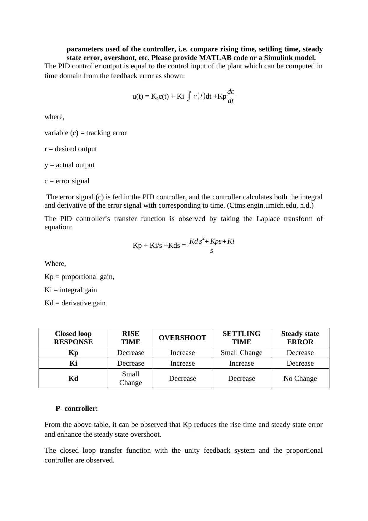
The PID controller output is equal to the control input of the plant which can be computed in
time domain from the feedback error as shown:
u(t) = Kpc(t) + Ki ∫ c(t)dt +Kp dc
dt
where,
variable (c) = tracking error
r = desired output
y = actual output
c = error signal
The error signal (c) is fed in the PID controller, and the controller calculates both the integral
and derivative of the error signal with corresponding to time. (Ctms.engin.umich.edu, n.d.)
The PID controller’s transfer function is observed by taking the Laplace transform of
equation:
Kp + Ki/s +Kds = Kd s2+ Kps+ Ki
s
Where,
Kp = proportional gain,
Ki = integral gain
Kd = derivative gain
Closed loop
RESPONSE
RISE
TIME OVERSHOOT SETTLING
TIME
Steady state
ERROR
Kp Decrease Increase Small Change Decrease
Ki Decrease Increase Increase Decrease
Kd Small
Change Decrease Decrease No Change
P- controller:
From the above table, it can be observed that Kp reduces the rise time and steady state error
and enhance the steady state overshoot.
The closed loop transfer function with the unity feedback system and the proportional
controller are observed.
state error, overshoot, etc. Please provide MATLAB code or a Simulink model.
The PID controller output is equal to the control input of the plant which can be computed in
time domain from the feedback error as shown:
u(t) = Kpc(t) + Ki ∫ c(t)dt +Kp dc
dt
where,
variable (c) = tracking error
r = desired output
y = actual output
c = error signal
The error signal (c) is fed in the PID controller, and the controller calculates both the integral
and derivative of the error signal with corresponding to time. (Ctms.engin.umich.edu, n.d.)
The PID controller’s transfer function is observed by taking the Laplace transform of
equation:
Kp + Ki/s +Kds = Kd s2+ Kps+ Ki
s
Where,
Kp = proportional gain,
Ki = integral gain
Kd = derivative gain
Closed loop
RESPONSE
RISE
TIME OVERSHOOT SETTLING
TIME
Steady state
ERROR
Kp Decrease Increase Small Change Decrease
Ki Decrease Increase Increase Decrease
Kd Small
Change Decrease Decrease No Change
P- controller:
From the above table, it can be observed that Kp reduces the rise time and steady state error
and enhance the steady state overshoot.
The closed loop transfer function with the unity feedback system and the proportional
controller are observed.
⊘ This is a preview!⊘
Do you want full access?
Subscribe today to unlock all pages.
Trusted by 1+ million students worldwide
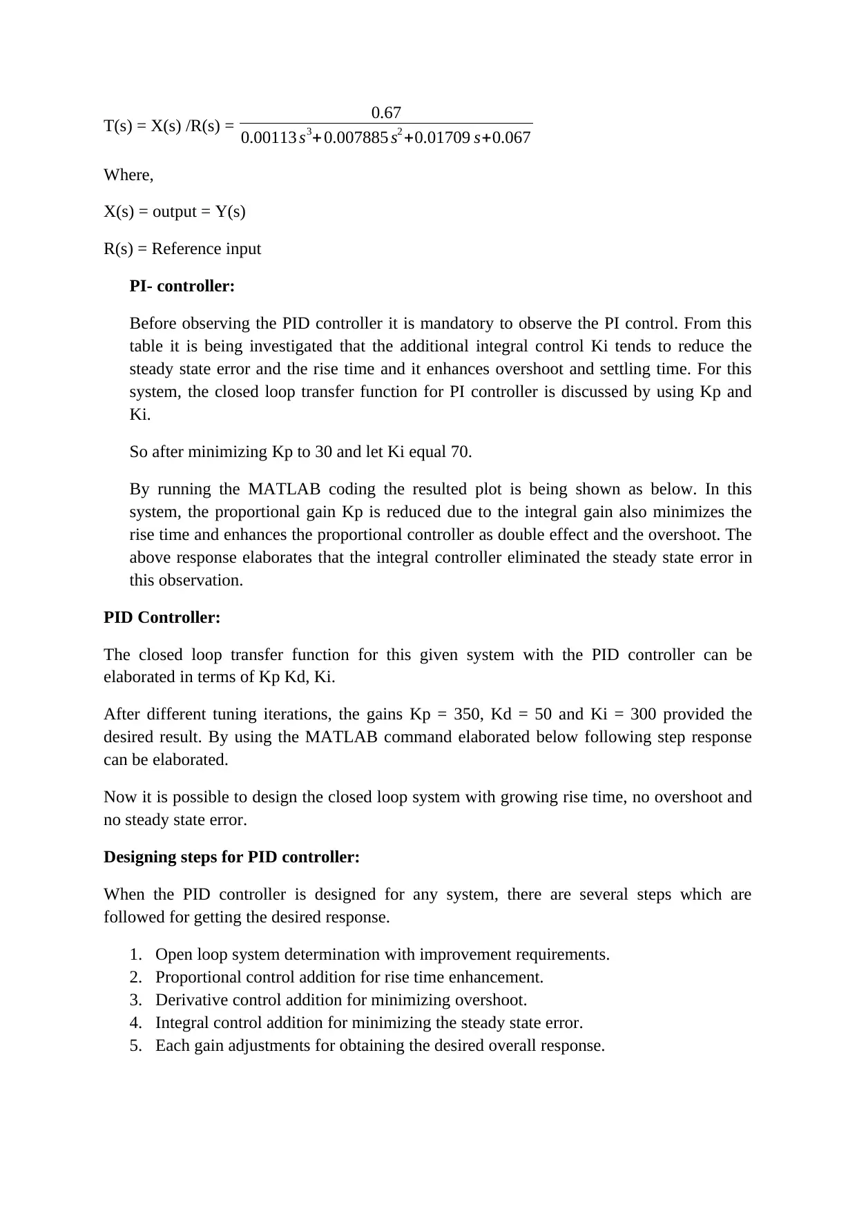
T(s) = X(s) /R(s) = 0.67
0.00113 s3+ 0.007885 s2 +0.01709 s+0.067
Where,
X(s) = output = Y(s)
R(s) = Reference input
PI- controller:
Before observing the PID controller it is mandatory to observe the PI control. From this
table it is being investigated that the additional integral control Ki tends to reduce the
steady state error and the rise time and it enhances overshoot and settling time. For this
system, the closed loop transfer function for PI controller is discussed by using Kp and
Ki.
So after minimizing Kp to 30 and let Ki equal 70.
By running the MATLAB coding the resulted plot is being shown as below. In this
system, the proportional gain Kp is reduced due to the integral gain also minimizes the
rise time and enhances the proportional controller as double effect and the overshoot. The
above response elaborates that the integral controller eliminated the steady state error in
this observation.
PID Controller:
The closed loop transfer function for this given system with the PID controller can be
elaborated in terms of Kp Kd, Ki.
After different tuning iterations, the gains Kp = 350, Kd = 50 and Ki = 300 provided the
desired result. By using the MATLAB command elaborated below following step response
can be elaborated.
Now it is possible to design the closed loop system with growing rise time, no overshoot and
no steady state error.
Designing steps for PID controller:
When the PID controller is designed for any system, there are several steps which are
followed for getting the desired response.
1. Open loop system determination with improvement requirements.
2. Proportional control addition for rise time enhancement.
3. Derivative control addition for minimizing overshoot.
4. Integral control addition for minimizing the steady state error.
5. Each gain adjustments for obtaining the desired overall response.
Paraphrase This Document
Need a fresh take? Get an instant paraphrase of this document with our AI Paraphraser
Appendices
PART:1
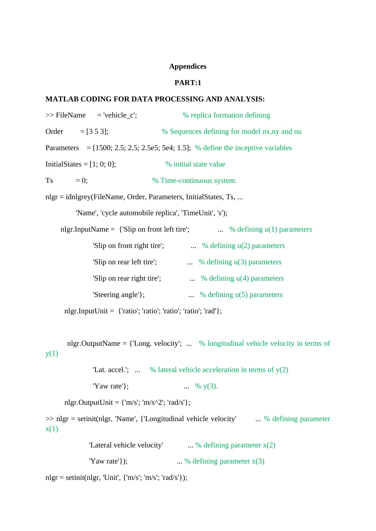
MATLAB CODING FOR DATA PROCESSING AND ANALYSIS:
>> FileName = 'vehicle_c'; % replica formation defining
Order = [3 5 3]; % Sequences defining for model nx,ny and nu
Parameters = [1500; 2.5; 2.5; 2.5e5; 5e4; 1.5]; % define the inceptive variables
InitialStates = [1; 0; 0]; % initial state value
Ts = 0; % Time-continuous system.
nlgr = idnlgrey(FileName, Order, Parameters, InitialStates, Ts, ...
'Name', 'cycle automobile replica', 'TimeUnit', 's');
nlgr.InputName = {'Slip on front left tire'; ... % defining u(1) parameters
'Slip on front right tire'; ... % defining u(2) parameters
'Slip on rear left tire'; ... % defining u(3) parameters
'Slip on rear right tire'; ... % defining u(4) parameters
'Steering angle'}; ... % defining u(5) parameters
nlgr.InputUnit = {'ratio'; 'ratio'; 'ratio'; 'ratio'; 'rad'};
nlgr.OutputName = {'Long. velocity'; ... % longitudinal vehicle velocity in terms of
y(1)
'Lat. accel.'; ... % lateral vehicle acceleration in terms of y(2)
'Yaw rate'}; ... % y(3).
nlgr.OutputUnit = {'m/s'; 'm/s^2'; 'rad/s'};
>> nlgr = setinit(nlgr, 'Name', {'Longitudinal vehicle velocity' ... % defining parameter
x(1)
'Lateral vehicle velocity' ... % defining parameter x(2)
'Yaw rate'}); ... % defining parameter x(3)
nlgr = setinit(nlgr, 'Unit', {'m/s'; 'm/s'; 'rad/s'});
PART:1
MATLAB CODING FOR DATA PROCESSING AND ANALYSIS:
>> FileName = 'vehicle_c'; % replica formation defining
Order = [3 5 3]; % Sequences defining for model nx,ny and nu
Parameters = [1500; 2.5; 2.5; 2.5e5; 5e4; 1.5]; % define the inceptive variables
InitialStates = [1; 0; 0]; % initial state value
Ts = 0; % Time-continuous system.
nlgr = idnlgrey(FileName, Order, Parameters, InitialStates, Ts, ...
'Name', 'cycle automobile replica', 'TimeUnit', 's');
nlgr.InputName = {'Slip on front left tire'; ... % defining u(1) parameters
'Slip on front right tire'; ... % defining u(2) parameters
'Slip on rear left tire'; ... % defining u(3) parameters
'Slip on rear right tire'; ... % defining u(4) parameters
'Steering angle'}; ... % defining u(5) parameters
nlgr.InputUnit = {'ratio'; 'ratio'; 'ratio'; 'ratio'; 'rad'};
nlgr.OutputName = {'Long. velocity'; ... % longitudinal vehicle velocity in terms of
y(1)
'Lat. accel.'; ... % lateral vehicle acceleration in terms of y(2)
'Yaw rate'}; ... % y(3).
nlgr.OutputUnit = {'m/s'; 'm/s^2'; 'rad/s'};
>> nlgr = setinit(nlgr, 'Name', {'Longitudinal vehicle velocity' ... % defining parameter
x(1)
'Lateral vehicle velocity' ... % defining parameter x(2)
'Yaw rate'}); ... % defining parameter x(3)
nlgr = setinit(nlgr, 'Unit', {'m/s'; 'm/s'; 'rad/s'});
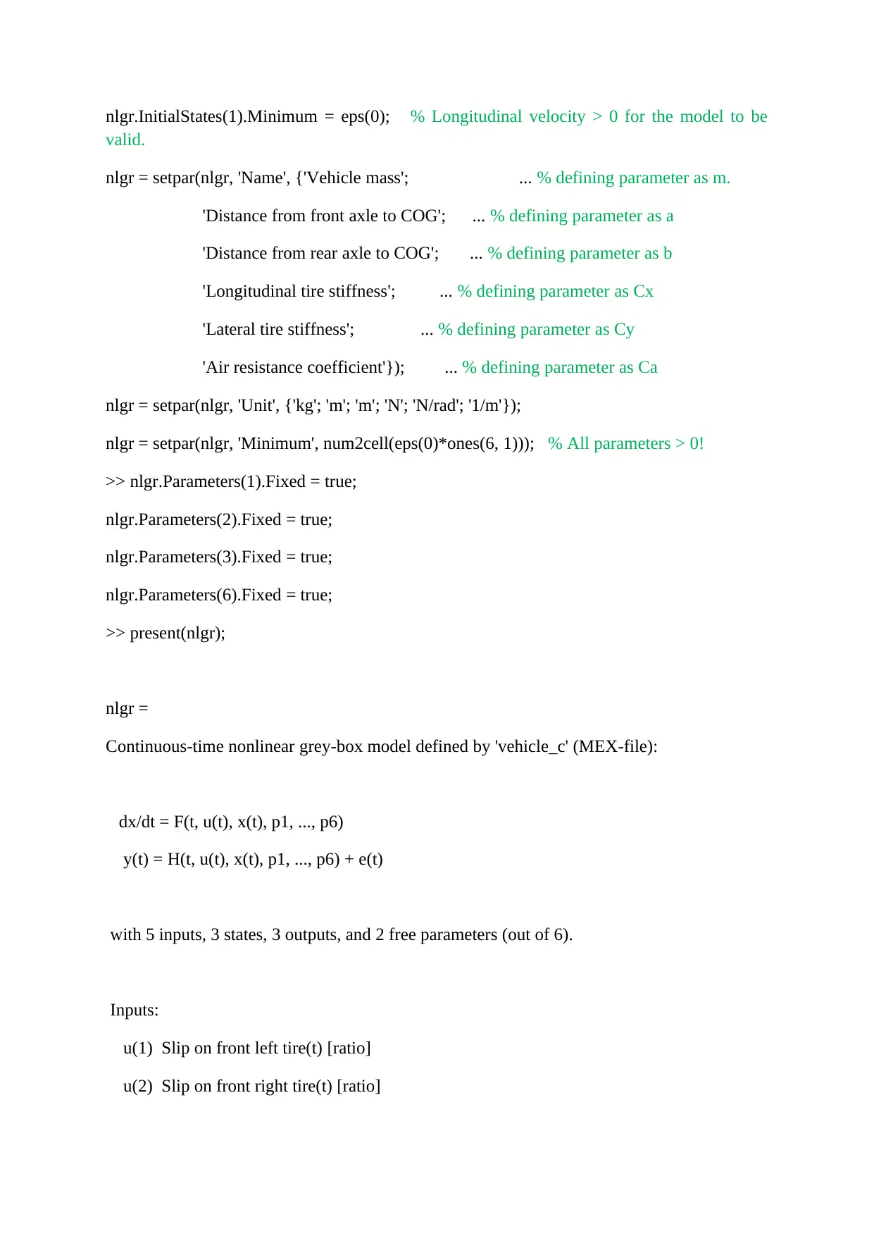
nlgr.InitialStates(1).Minimum = eps(0); % Longitudinal velocity > 0 for the model to be
valid.
nlgr = setpar(nlgr, 'Name', {'Vehicle mass'; ... % defining parameter as m.
'Distance from front axle to COG'; ... % defining parameter as a
'Distance from rear axle to COG'; ... % defining parameter as b
'Longitudinal tire stiffness'; ... % defining parameter as Cx
'Lateral tire stiffness'; ... % defining parameter as Cy
'Air resistance coefficient'}); ... % defining parameter as Ca
nlgr = setpar(nlgr, 'Unit', {'kg'; 'm'; 'm'; 'N'; 'N/rad'; '1/m'});
nlgr = setpar(nlgr, 'Minimum', num2cell(eps(0)*ones(6, 1))); % All parameters > 0!
>> nlgr.Parameters(1).Fixed = true;
nlgr.Parameters(2).Fixed = true;
nlgr.Parameters(3).Fixed = true;
nlgr.Parameters(6).Fixed = true;
>> present(nlgr);
nlgr =
Continuous-time nonlinear grey-box model defined by 'vehicle_c' (MEX-file):
dx/dt = F(t, u(t), x(t), p1, ..., p6)
y(t) = H(t, u(t), x(t), p1, ..., p6) + e(t)
with 5 inputs, 3 states, 3 outputs, and 2 free parameters (out of 6).
Inputs:
u(1) Slip on front left tire(t) [ratio]
u(2) Slip on front right tire(t) [ratio]
⊘ This is a preview!⊘
Do you want full access?
Subscribe today to unlock all pages.
Trusted by 1+ million students worldwide
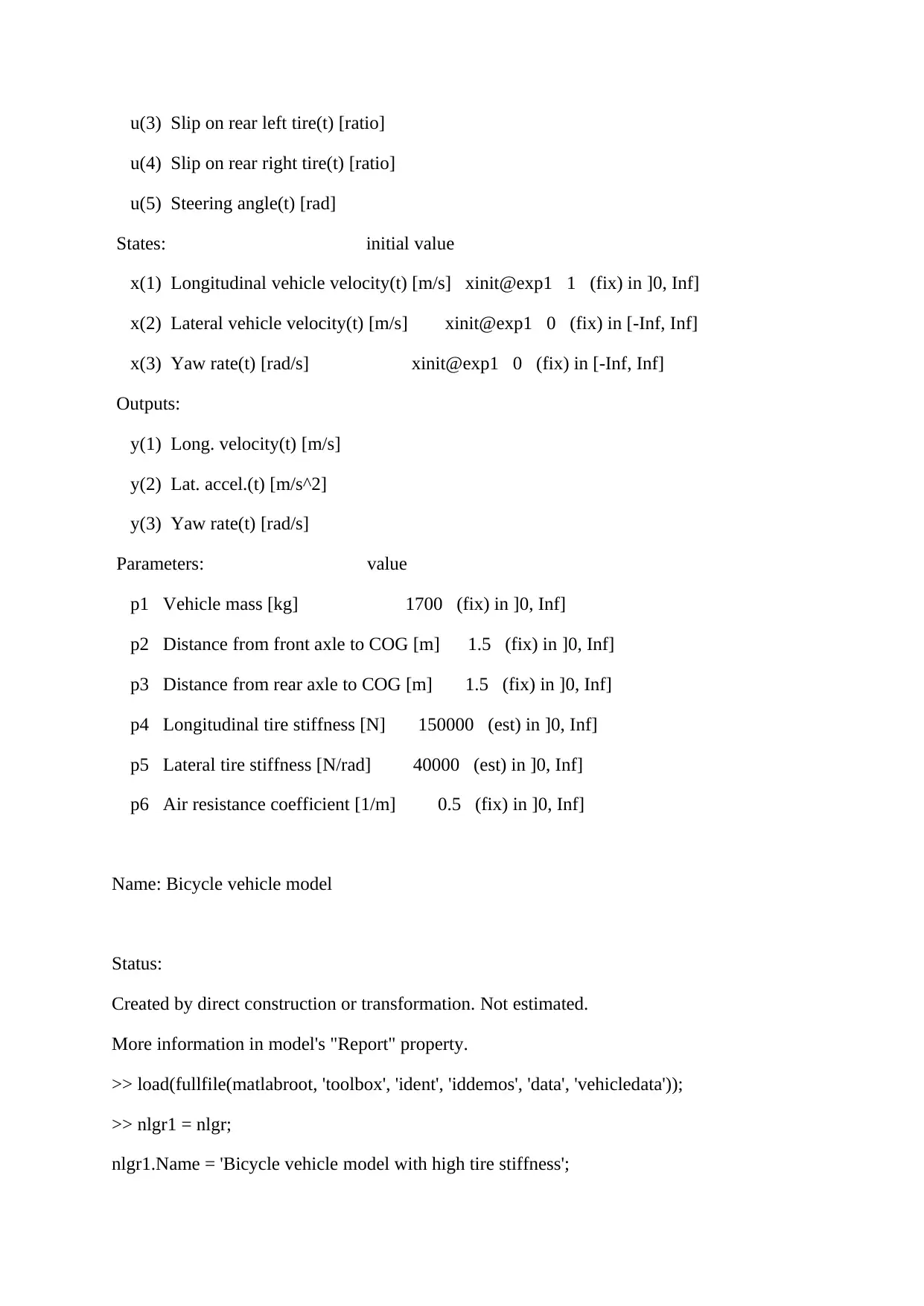
u(3) Slip on rear left tire(t) [ratio]
u(4) Slip on rear right tire(t) [ratio]
u(5) Steering angle(t) [rad]
States: initial value
x(1) Longitudinal vehicle velocity(t) [m/s] xinit@exp1 1 (fix) in ]0, Inf]
x(2) Lateral vehicle velocity(t) [m/s] xinit@exp1 0 (fix) in [-Inf, Inf]
x(3) Yaw rate(t) [rad/s] xinit@exp1 0 (fix) in [-Inf, Inf]
Outputs:
y(1) Long. velocity(t) [m/s]
y(2) Lat. accel.(t) [m/s^2]
y(3) Yaw rate(t) [rad/s]
Parameters: value
p1 Vehicle mass [kg] 1700 (fix) in ]0, Inf]
p2 Distance from front axle to COG [m] 1.5 (fix) in ]0, Inf]
p3 Distance from rear axle to COG [m] 1.5 (fix) in ]0, Inf]
p4 Longitudinal tire stiffness [N] 150000 (est) in ]0, Inf]
p5 Lateral tire stiffness [N/rad] 40000 (est) in ]0, Inf]
p6 Air resistance coefficient [1/m] 0.5 (fix) in ]0, Inf]
Name: Bicycle vehicle model
Status:
Created by direct construction or transformation. Not estimated.
More information in model's "Report" property.
>> load(fullfile(matlabroot, 'toolbox', 'ident', 'iddemos', 'data', 'vehicledata'));
>> nlgr1 = nlgr;
nlgr1.Name = 'Bicycle vehicle model with high tire stiffness';
Paraphrase This Document
Need a fresh take? Get an instant paraphrase of this document with our AI Paraphraser
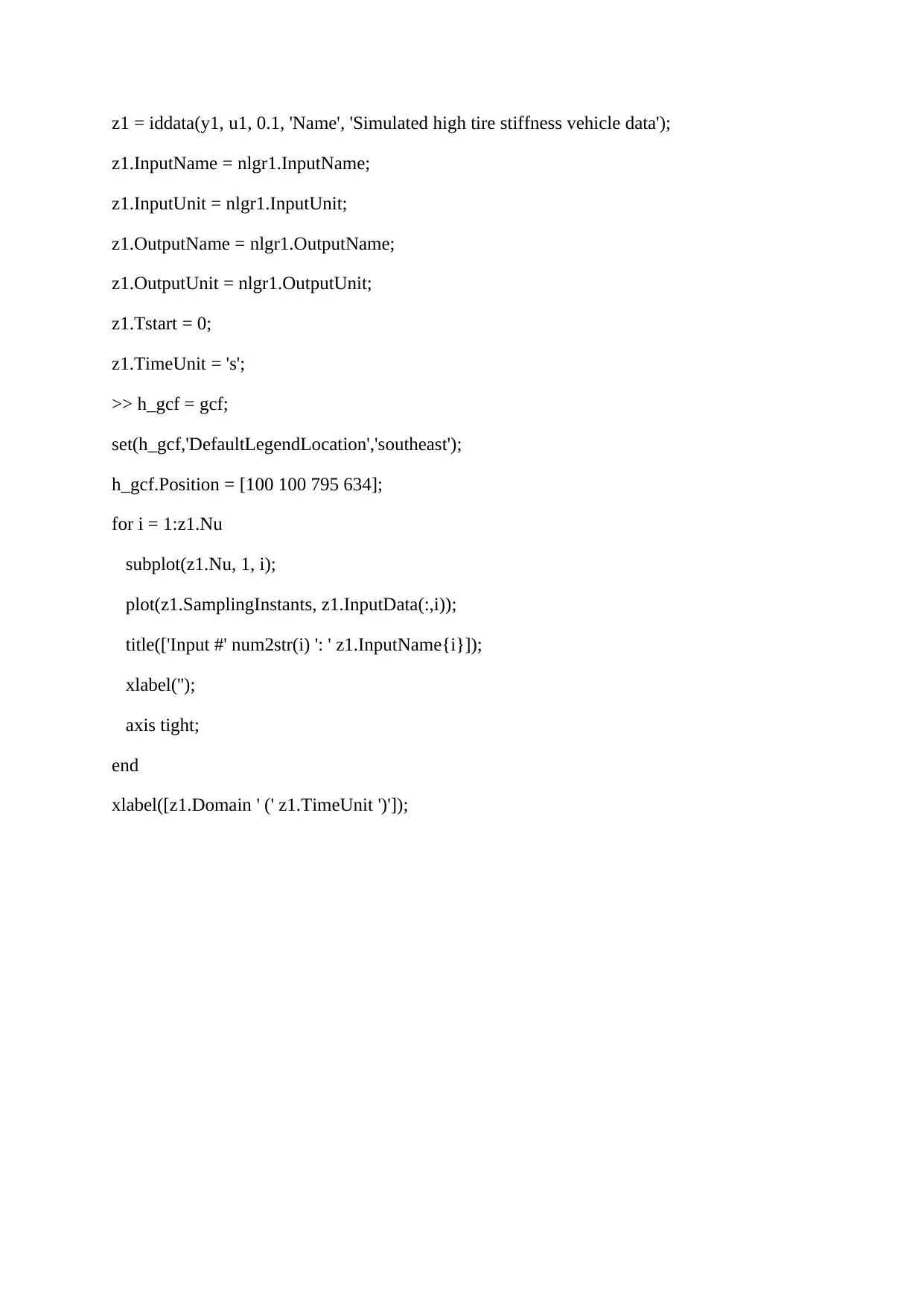
z1 = iddata(y1, u1, 0.1, 'Name', 'Simulated high tire stiffness vehicle data');
z1.InputName = nlgr1.InputName;
z1.InputUnit = nlgr1.InputUnit;
z1.OutputName = nlgr1.OutputName;
z1.OutputUnit = nlgr1.OutputUnit;
z1.Tstart = 0;
z1.TimeUnit = 's';
>> h_gcf = gcf;
set(h_gcf,'DefaultLegendLocation','southeast');
h_gcf.Position = [100 100 795 634];
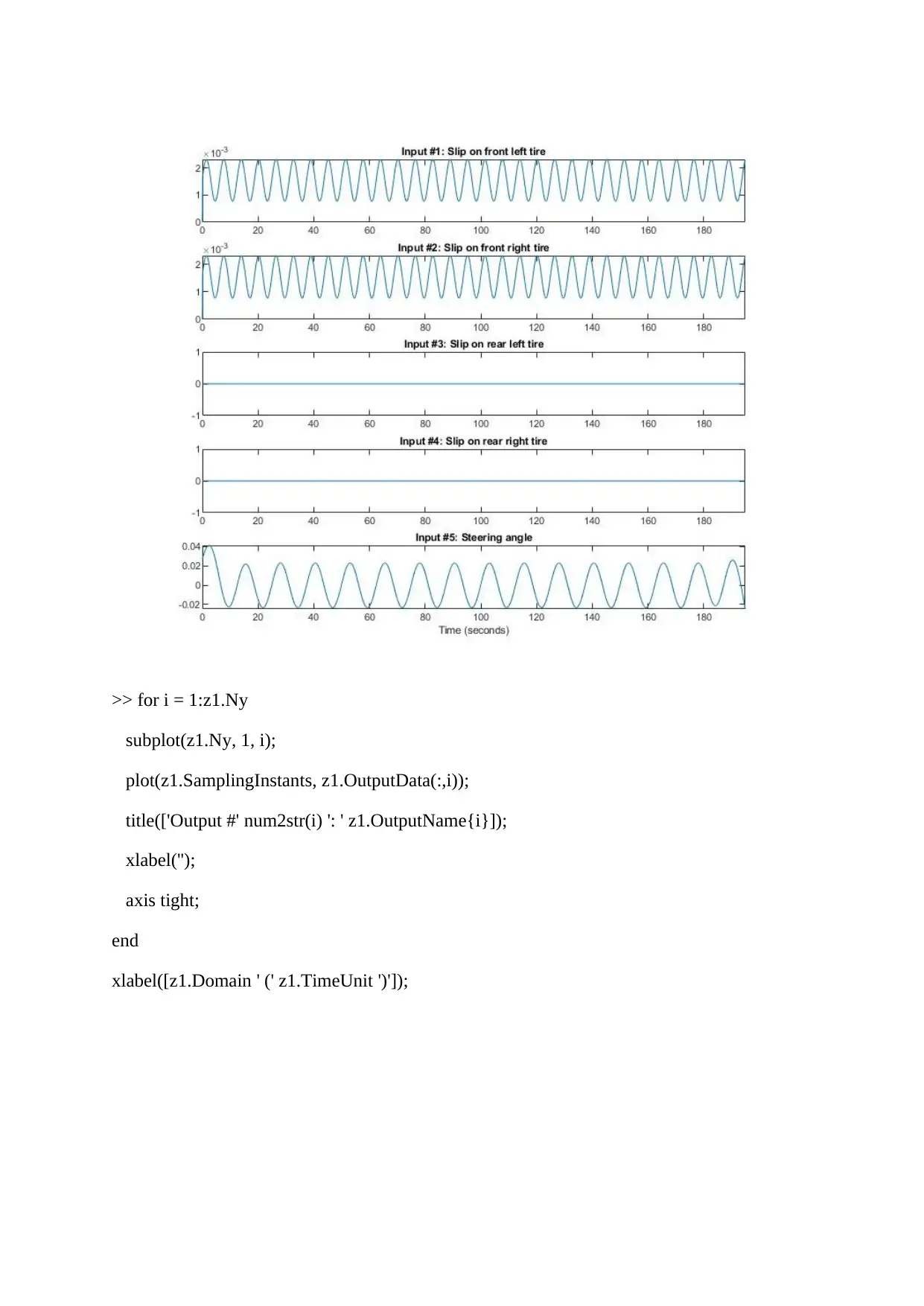
for i = 1:z1.Nu
subplot(z1.Nu, 1, i);
plot(z1.SamplingInstants, z1.InputData(:,i));
title(['Input #' num2str(i) ': ' z1.InputName{i}]);
xlabel('');
axis tight;
end
xlabel([z1.Domain ' (' z1.TimeUnit ')']);
z1.InputName = nlgr1.InputName;
z1.InputUnit = nlgr1.InputUnit;
z1.OutputName = nlgr1.OutputName;
z1.OutputUnit = nlgr1.OutputUnit;
z1.Tstart = 0;
z1.TimeUnit = 's';
>> h_gcf = gcf;
set(h_gcf,'DefaultLegendLocation','southeast');
h_gcf.Position = [100 100 795 634];
for i = 1:z1.Nu
subplot(z1.Nu, 1, i);
plot(z1.SamplingInstants, z1.InputData(:,i));
title(['Input #' num2str(i) ': ' z1.InputName{i}]);
xlabel('');
axis tight;
end
xlabel([z1.Domain ' (' z1.TimeUnit ')']);
>> for i = 1:z1.Ny
subplot(z1.Ny, 1, i);
plot(z1.SamplingInstants, z1.OutputData(:,i));
title(['Output #' num2str(i) ': ' z1.OutputName{i}]);
xlabel('');
axis tight;
end
xlabel([z1.Domain ' (' z1.TimeUnit ')']);
subplot(z1.Ny, 1, i);
plot(z1.SamplingInstants, z1.OutputData(:,i));
title(['Output #' num2str(i) ': ' z1.OutputName{i}]);
xlabel('');
axis tight;
end
xlabel([z1.Domain ' (' z1.TimeUnit ')']);
⊘ This is a preview!⊘
Do you want full access?
Subscribe today to unlock all pages.
Trusted by 1+ million students worldwide
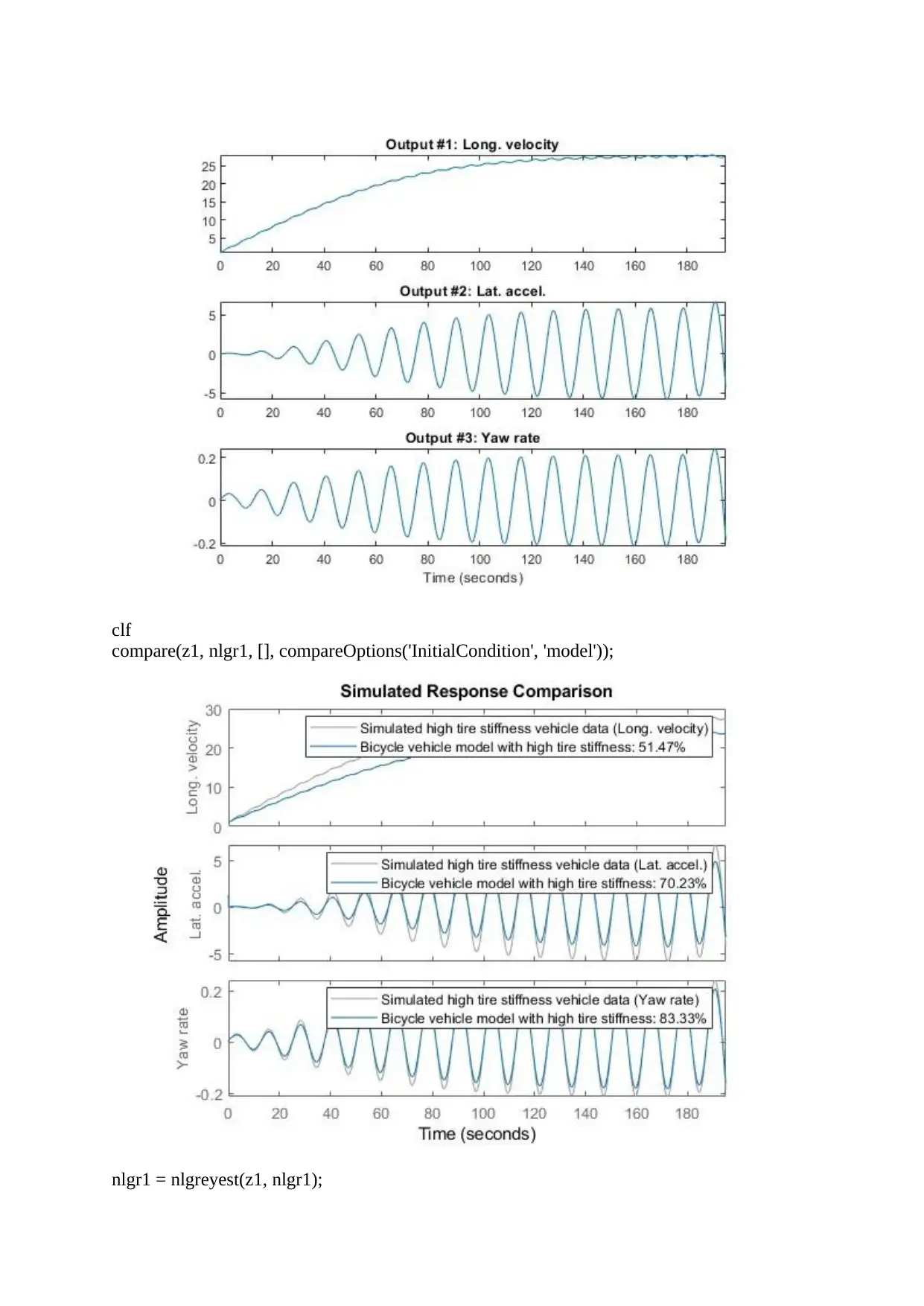
clf
compare(z1, nlgr1, [], compareOptions('InitialCondition', 'model'));
nlgr1 = nlgreyest(z1, nlgr1);
compare(z1, nlgr1, [], compareOptions('InitialCondition', 'model'));
nlgr1 = nlgreyest(z1, nlgr1);
Paraphrase This Document
Need a fresh take? Get an instant paraphrase of this document with our AI Paraphraser
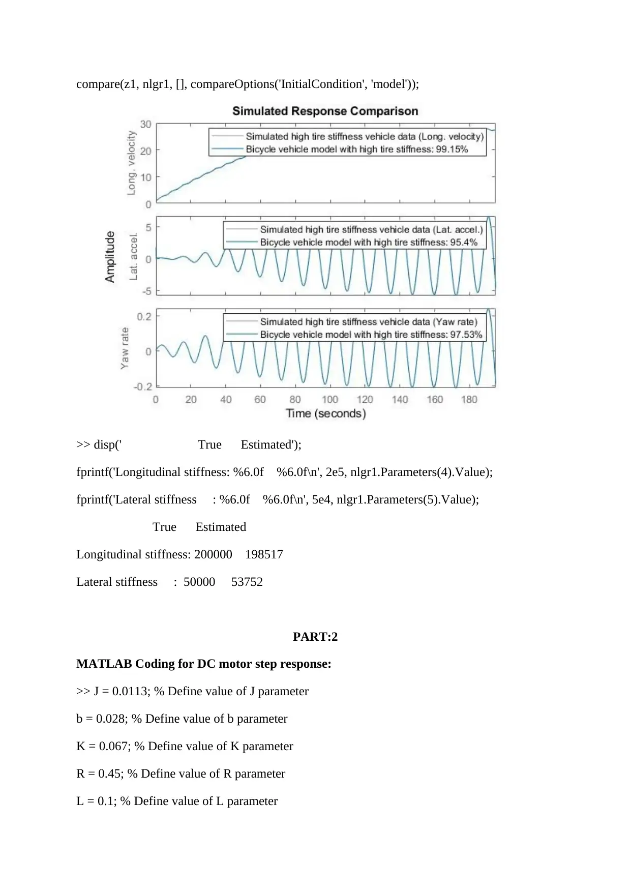
compare(z1, nlgr1, [], compareOptions('InitialCondition', 'model'));
>> disp(' True Estimated');
fprintf('Longitudinal stiffness: %6.0f %6.0f\n', 2e5, nlgr1.Parameters(4).Value);
fprintf('Lateral stiffness : %6.0f %6.0f\n', 5e4, nlgr1.Parameters(5).Value);
True Estimated
Longitudinal stiffness: 200000 198517
Lateral stiffness : 50000 53752
PART:2
MATLAB Coding for DC motor step response:
>> J = 0.0113; % Define value of J parameter
b = 0.028; % Define value of b parameter
K = 0.067; % Define value of K parameter
R = 0.45; % Define value of R parameter
L = 0.1; % Define value of L parameter
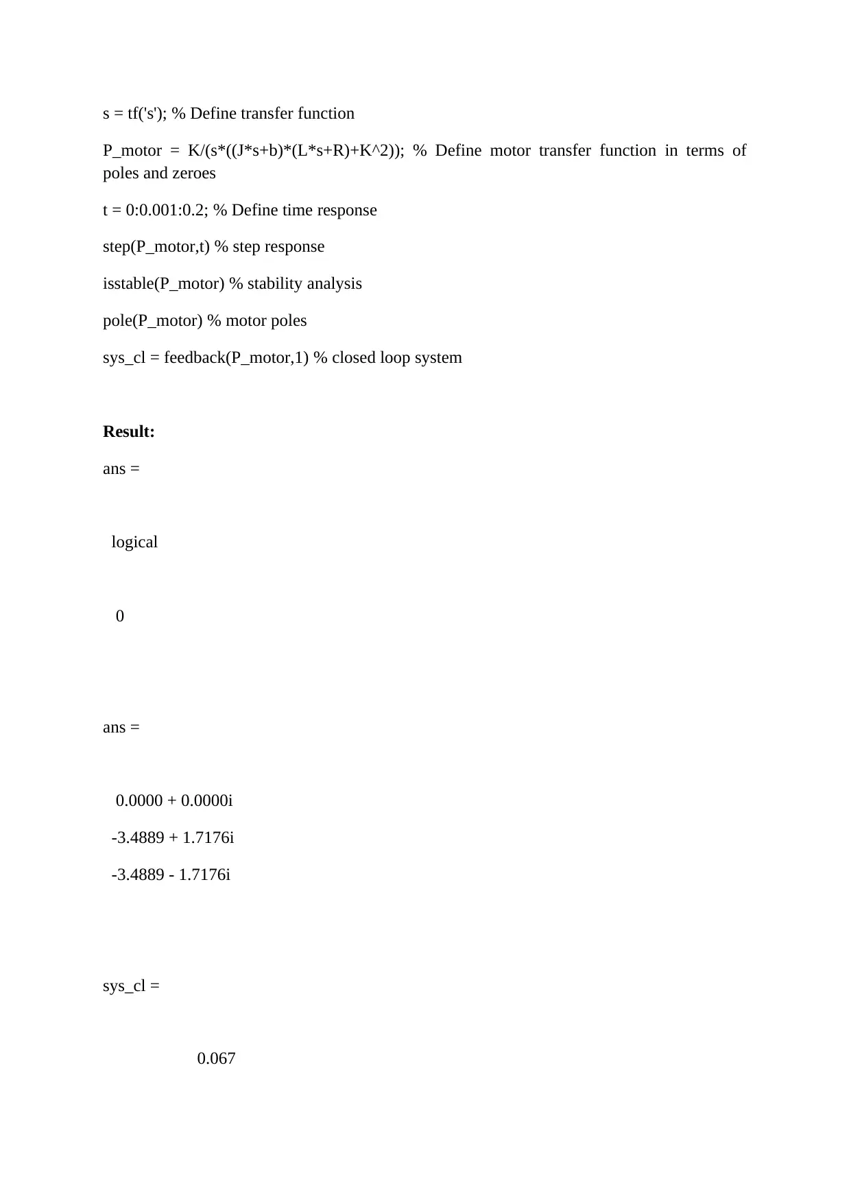
s = tf('s'); % Define transfer function
P_motor = K/(s*((J*s+b)*(L*s+R)+K^2)); % Define motor transfer function in terms of
poles and zeroes
t = 0:0.001:0.2; % Define time response
step(P_motor,t) % step response
isstable(P_motor) % stability analysis
pole(P_motor) % motor poles
sys_cl = feedback(P_motor,1) % closed loop system
Result:
ans =
logical
0
ans =
0.0000 + 0.0000i
-3.4889 + 1.7176i
-3.4889 - 1.7176i
sys_cl =
0.067
⊘ This is a preview!⊘
Do you want full access?
Subscribe today to unlock all pages.
Trusted by 1+ million students worldwide
1 out of 22

Your All-in-One AI-Powered Toolkit for Academic Success.
+13062052269
info@desklib.com
Available 24*7 on WhatsApp / Email
![[object Object]](/_next/static/media/star-bottom.7253800d.svg)
Unlock your academic potential
Copyright © 2020–2026 A2Z Services. All Rights Reserved. Developed and managed by ZUCOL.