Deakin University: Real World Analytics Project - Heating and Cooling

This project analyzes heating and cooling loads in buildings, focusing on the relationship between building characteristics and energy consumption. The analysis uses data from 768 simulated buildings, examining variables such as relative compactness, surface area, wall area, roof area, and overall height. The study explores these variables' impact on heating load (Y1) and cooling load (Y2). The project utilizes R for data exploration, including histograms and scatter plots to visualize relationships. It then assesses the performance of various models, including weighted average, weighted power means, ordered weighted average, and Choquet's integral, in predicting heating load. The weighted power mean model with a power of 0.5 is identified as the best fit. Finally, a multiple regression analysis is performed to predict heating load based on selected independent variables, concluding with a predicted value and an evaluation of the model's coefficients and statistical significance.

Running head: REAL WORLD ANALYTICS
REAL WORLD ANALYTICS
Name of Student
Name of University

1REAL WORLD ANALYTICS
Table of Contents
Part A:..............................................................................................................................................2
Description of Data......................................................................................................................2
Task 1...........................................................................................................................................2
Task 2.........................................................................................................................................10
Task 3.........................................................................................................................................10
Task 4.........................................................................................................................................11

2REAL WORLD ANALYTICS
Part A:
Description of Data
Heating and cooling load are quite significant consideration while determining the
specifics of the equipment used for heating and cooling purposes in eco-friendly , energy saving
designs of buildings. It is why tools used for simulation of energy for predicting the tentative
energy consumption behavior in a building are necessary.
The paper considers the two parameters, Heating load (Y1) and Cooling load (Y2) as
variables of interest to be studied and analyzed. The study takes into account the independent
variables such as relative compactness (X1), Surface area (X2), wall area (X3), roof area (X4)
and additionally the overall height (X5) of the building as indicators or influencers of the two
variables heating load and cooling load. The data consists of data from 768 buildings which was
simulated via building simulator tool. The subsequent analysis as per the requirements of the
assignment was done in R.
Task 1
The file ENB18data.txt, downloaded from CloudDeakin consists of the data as described
in the previous section which was used for the study. The data was saved in the working
directory of R software and thus loaded into R environment. It was assigned to a data matrix,
named “the.data” as directed by the requirement file of the assignment. The matrix had 7
columns storing data on the seven variables and 786 rows of observations on each of the seven
variables.
The assignment required only one variable of interest to be chosen between the heating
Load (Y1) and the cooling load (Y2). Y1 was chosen as the study variable for this paper. Thus
this the paper deals with the analysis of the Y1 variable and its relationship with the other
independent variables X1, X2, X3, X4, and X5. A sample of size 300 was chosen randomly from
among the 768 rows of data, as directed by the assignment requirements and the ensuing analysis
was done on this sample.
The following diagram shows the histogram of the variable Y1 or annual heating load
(KWh / meter square). It is seen to follow a distribution which is positively skewed , which
means that most of the values of Y1 seem to be located along the left hand side of the
distributional curve or the left tail which makes its right tail more elongated than its left making
it positively or right skewed. The mode or the maximum frequency is found to be in the interval
between 15KWh per square meter and 20KWh per square meter.

3REAL WORLD ANALYTICS
Figure 1
The value of the variable X1 or relative compactness values more or less lie around the
center of the distribution in the interval between 0.6% and 1%.

4REAL WORLD ANALYTICS
Figure 2
The surface area was found to be symmetrically distributed. However there exists a slight
skew to the distribution towards the lower tails making it slightly positively skewed. The highest
frequency or the mode was observed to be in the interval between 600 and 650 squared meter.
Figure 3
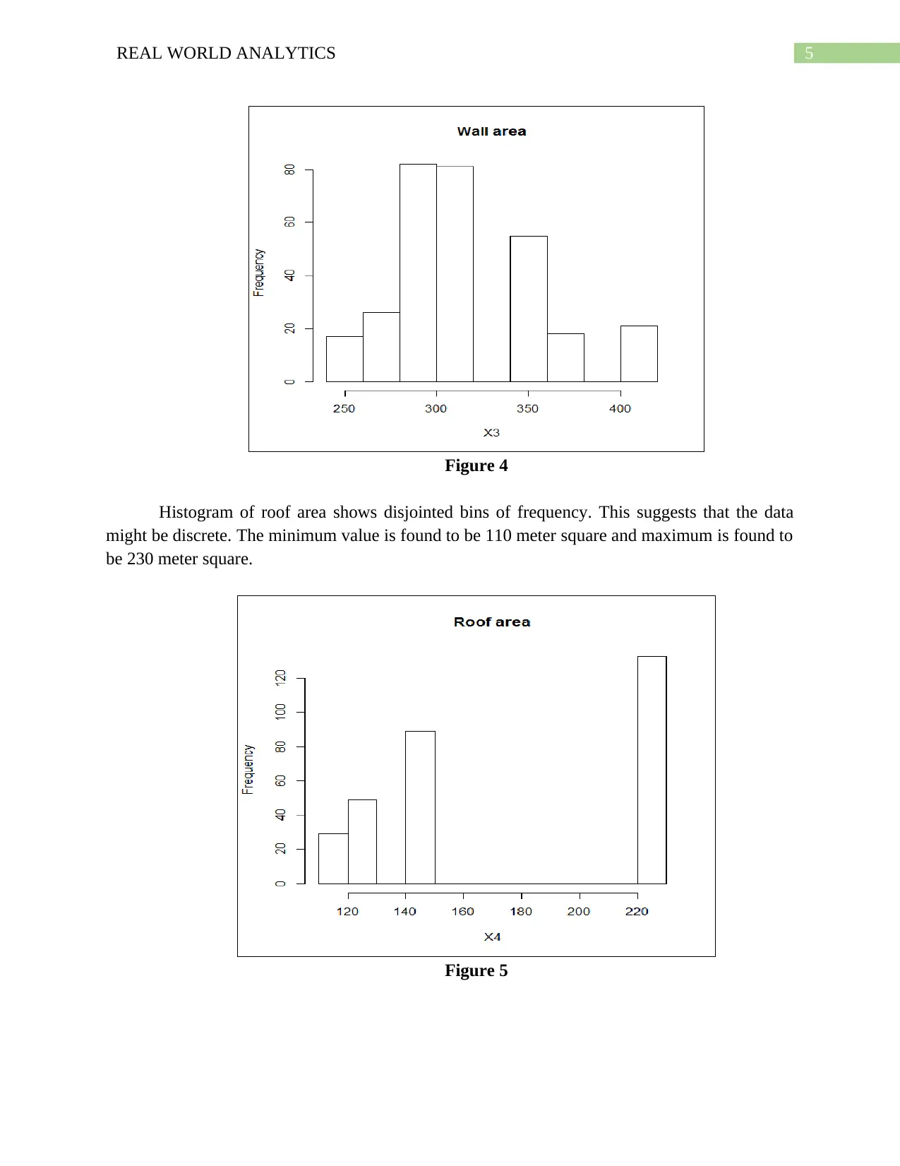
The histogram of the wall area shows a right skewed or positively skewed distribution
with its values lying between 200 square meters and 500 square meters. The modal class was
identified as the interval between 290 square meter to 300 square meter.

5REAL WORLD ANALYTICS
Figure 4
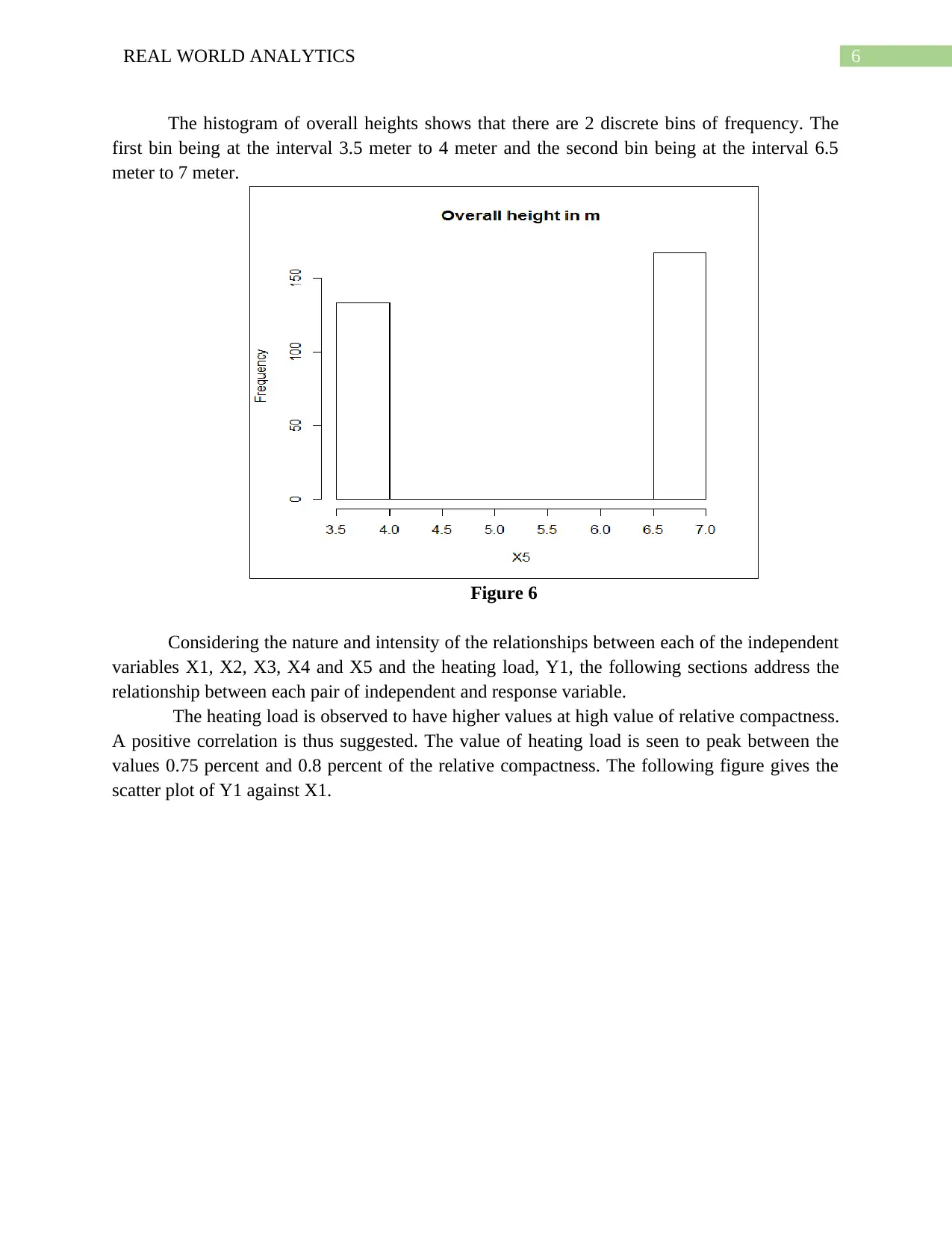
Histogram of roof area shows disjointed bins of frequency. This suggests that the data
might be discrete. The minimum value is found to be 110 meter square and maximum is found to
be 230 meter square.
Figure 5

6REAL WORLD ANALYTICS
The histogram of overall heights shows that there are 2 discrete bins of frequency. The
first bin being at the interval 3.5 meter to 4 meter and the second bin being at the interval 6.5
meter to 7 meter.
Figure 6
Considering the nature and intensity of the relationships between each of the independent
variables X1, X2, X3, X4 and X5 and the heating load, Y1, the following sections address the
relationship between each pair of independent and response variable.
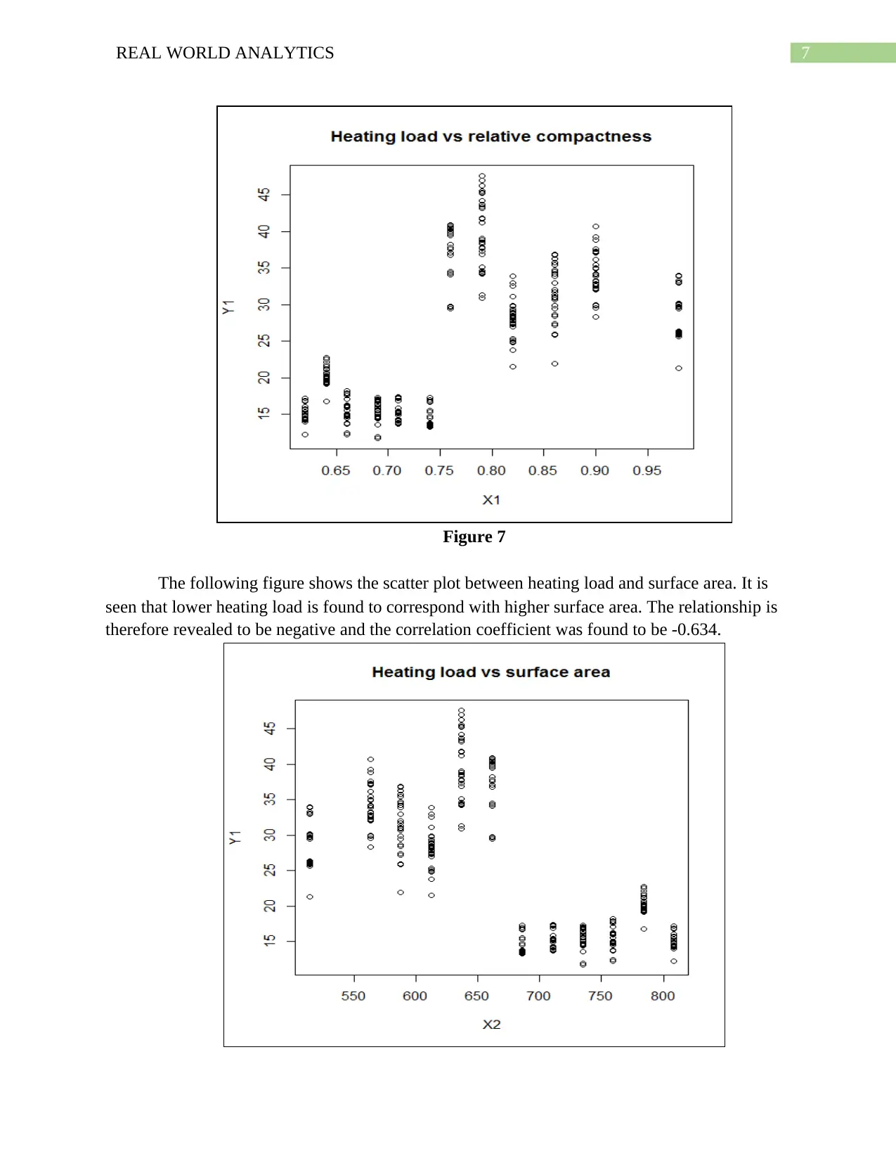
The heating load is observed to have higher values at high value of relative compactness.
A positive correlation is thus suggested. The value of heating load is seen to peak between the
values 0.75 percent and 0.8 percent of the relative compactness. The following figure gives the
scatter plot of Y1 against X1.

7REAL WORLD ANALYTICS
Figure 7
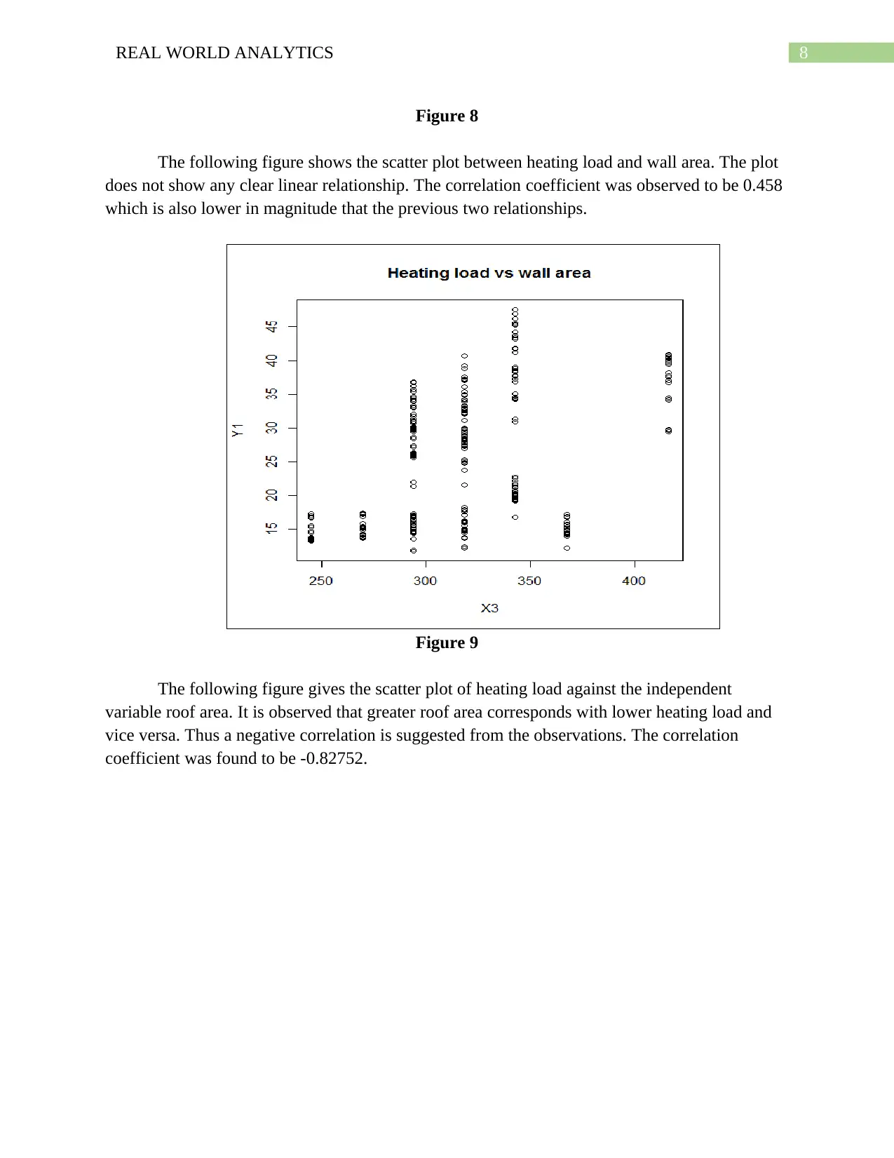
The following figure shows the scatter plot between heating load and surface area. It is
seen that lower heating load is found to correspond with higher surface area. The relationship is
therefore revealed to be negative and the correlation coefficient was found to be -0.634.

8REAL WORLD ANALYTICS
Figure 8
The following figure shows the scatter plot between heating load and wall area. The plot
does not show any clear linear relationship. The correlation coefficient was observed to be 0.458
which is also lower in magnitude that the previous two relationships.
Figure 9
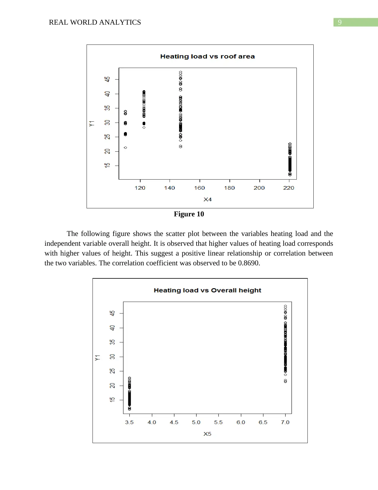
The following figure gives the scatter plot of heating load against the independent
variable roof area. It is observed that greater roof area corresponds with lower heating load and
vice versa. Thus a negative correlation is suggested from the observations. The correlation
coefficient was found to be -0.82752.

9REAL WORLD ANALYTICS
Figure 10
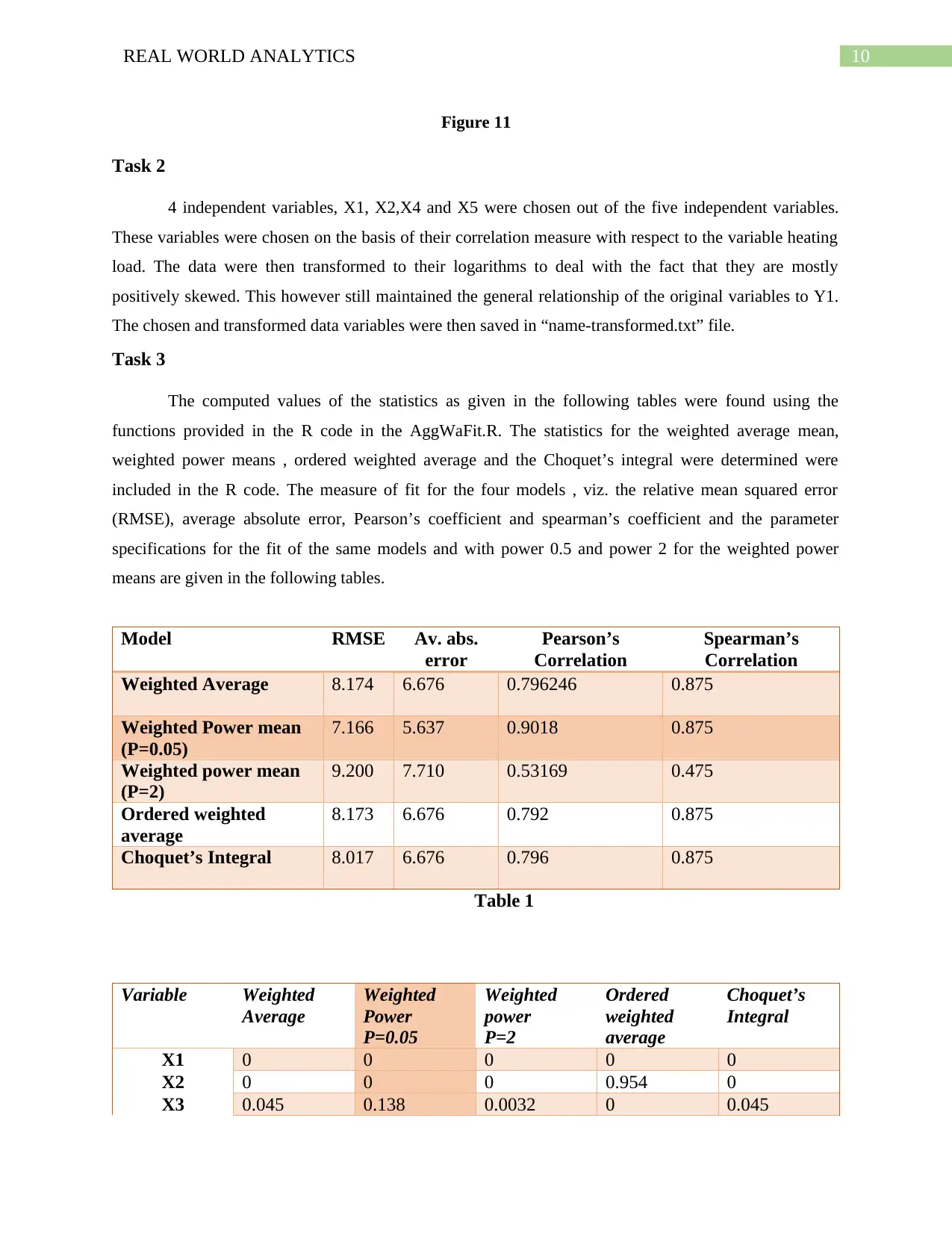
The following figure shows the scatter plot between the variables heating load and the
independent variable overall height. It is observed that higher values of heating load corresponds
with higher values of height. This suggest a positive linear relationship or correlation between
the two variables. The correlation coefficient was observed to be 0.8690.

10REAL WORLD ANALYTICS
Figure 11
Task 2
4 independent variables, X1, X2,X4 and X5 were chosen out of the five independent variables.
These variables were chosen on the basis of their correlation measure with respect to the variable heating
load. The data were then transformed to their logarithms to deal with the fact that they are mostly
positively skewed. This however still maintained the general relationship of the original variables to Y1.
The chosen and transformed data variables were then saved in “name-transformed.txt” file.
Task 3
The computed values of the statistics as given in the following tables were found using the
functions provided in the R code in the AggWaFit.R. The statistics for the weighted average mean,
weighted power means , ordered weighted average and the Choquet’s integral were determined were
included in the R code. The measure of fit for the four models , viz. the relative mean squared error
(RMSE), average absolute error, Pearson’s coefficient and spearman’s coefficient and the parameter
specifications for the fit of the same models and with power 0.5 and power 2 for the weighted power
means are given in the following tables.
Model RMSE Av. abs.
error
Pearson’s
Correlation
Spearman’s
Correlation
Weighted Average 8.174 6.676 0.796246 0.875
Weighted Power mean
(P=0.05)
7.166 5.637 0.9018 0.875
Weighted power mean
(P=2)
9.200 7.710 0.53169 0.475
Ordered weighted
average
8.173 6.676 0.792 0.875
Choquet’s Integral 8.017 6.676 0.796 0.875
Table 1
Variable Weighted
Average
Weighted
Power
P=0.05
Weighted
power
P=2
Ordered
weighted
average
Choquet’s
Integral
X1 0 0 0 0 0
X2 0 0 0 0.954 0
X3 0.045 0.138 0.0032 0 0.045

11REAL WORLD ANALYTICS
X4 0 0 0 0.045 0
X5 0.9549 0.861 0.9967 0 0.954
Table 2
The model which was found to have the best specifications with least error and maximum
correlation values was the weighted power mean model with the power parameter being 0.5.
The weighted power model with power 0.5 revealed that wall area and overall height
have the most weightage, in fact the only weightage on the heating load. The weights are positive
and hence the greater are the values of X3 and X5, greater is the heating load as per the weighted
power model with power 0.5.
Task 4
Making use of the four variables that were identified and stored in “name-transformed.txt”
after logarithmic conversion, the altered independent variables were applied to a regression analysis with
respect to heating load Y1.Thus a multiple regression analysis was done via R with Y1 on the logarithms
of the variables X1, X2, X4 and X5. The variable found to be significant were all X1, X2, X4 and X5.
Plugging in the given values of X1 equals to 0.82, X2 equals to 612.5, X3 equals to 318.5, X4 equals to
147, and X5 equals to 7, the predicted value of logarithm of Y1 after having been transformed to Y1 was
computed as 28.42.
Unit increase in values of the variables logarithm of X1, X2, and X5 was seen correspond with
increase of 777, 9.799 and 1.45 units in logarithm of heating load respectively whereas for X4 it was a
decrease of 0.6087 per unit increase. The predicted value of Y1 was found to lie within the range of
value of observed Y1 and the adjusted R squared if the model was high at 0.8459 and the result of the
model which is the predicted Y1 was therefore considered likely.
Coefficients:
Estimate Std. Error t value Pr(>|t|)
(Intercept) -57.74448 20.75804 -2.782 0.00575 **
Xt1 7.77801 3.21154 2.422 0.01604 *
Xt2 9.79958 3.35725 2.919 0.00378 **
Xt4 -0.60876 0.15432 -3.945 9.98e-05 ***
Xt5 1.45068 0.09803 14.798 < 2e-16 ***
---
Signif. codes: 0 ‘***’ 0.001 ‘**’ 0.01 ‘*’ 0.05 ‘.’ 0.1 ‘ ’ 1