Deakin University SIT718: Assessment 3 - Aggregation Function Analysis

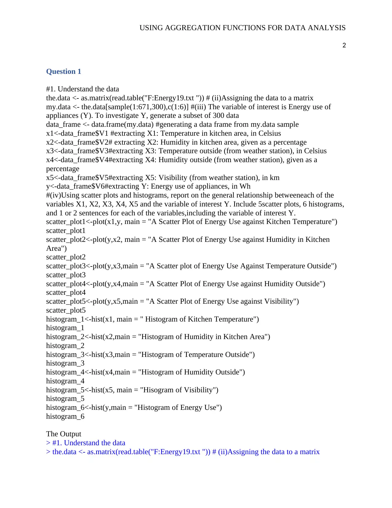
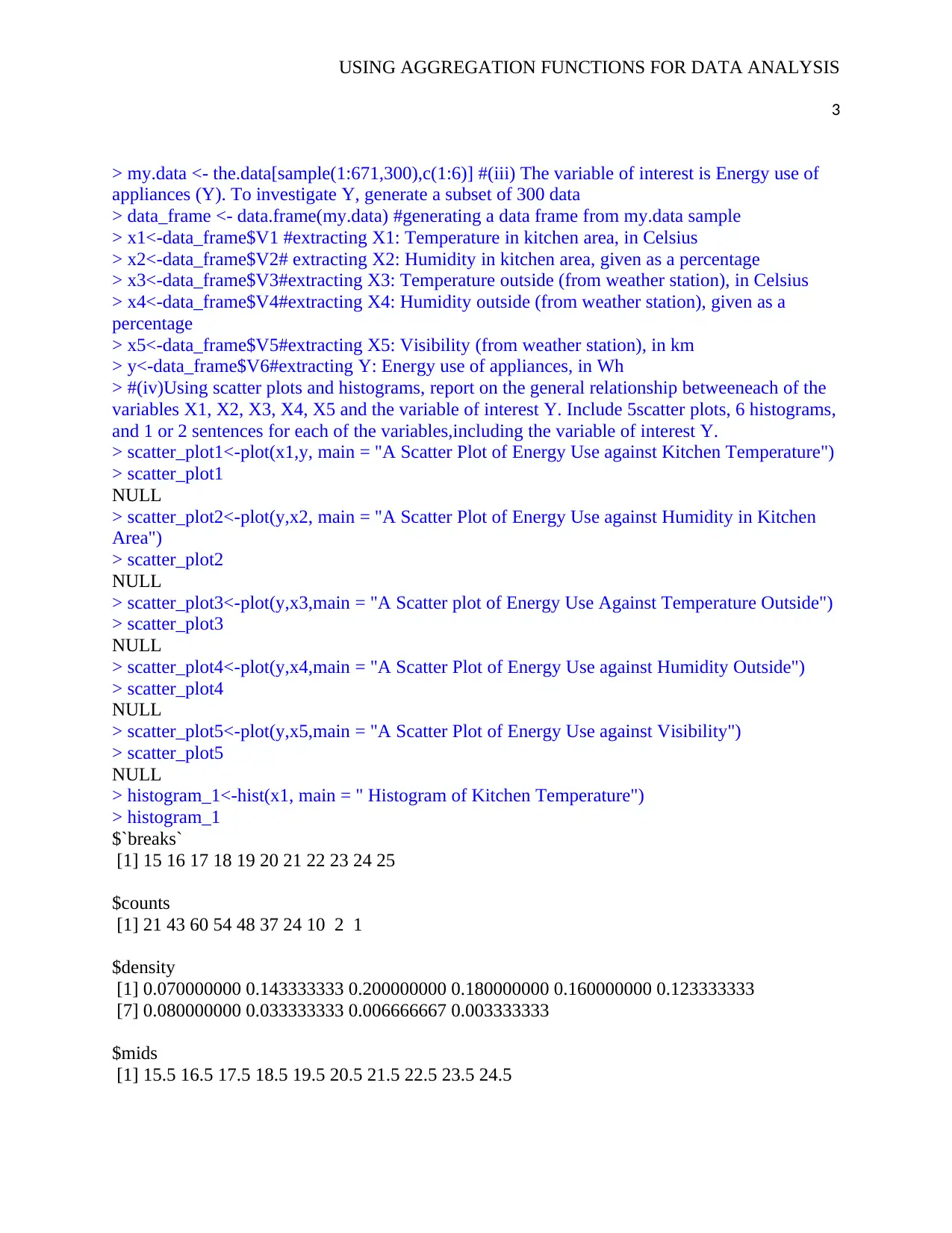
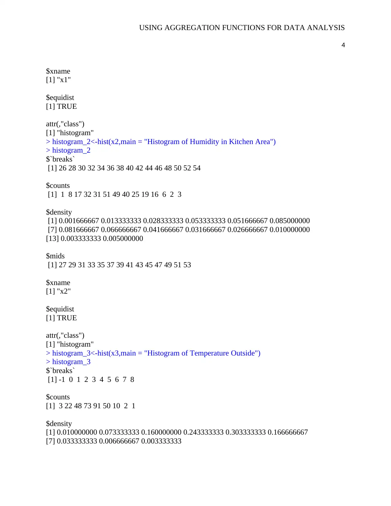
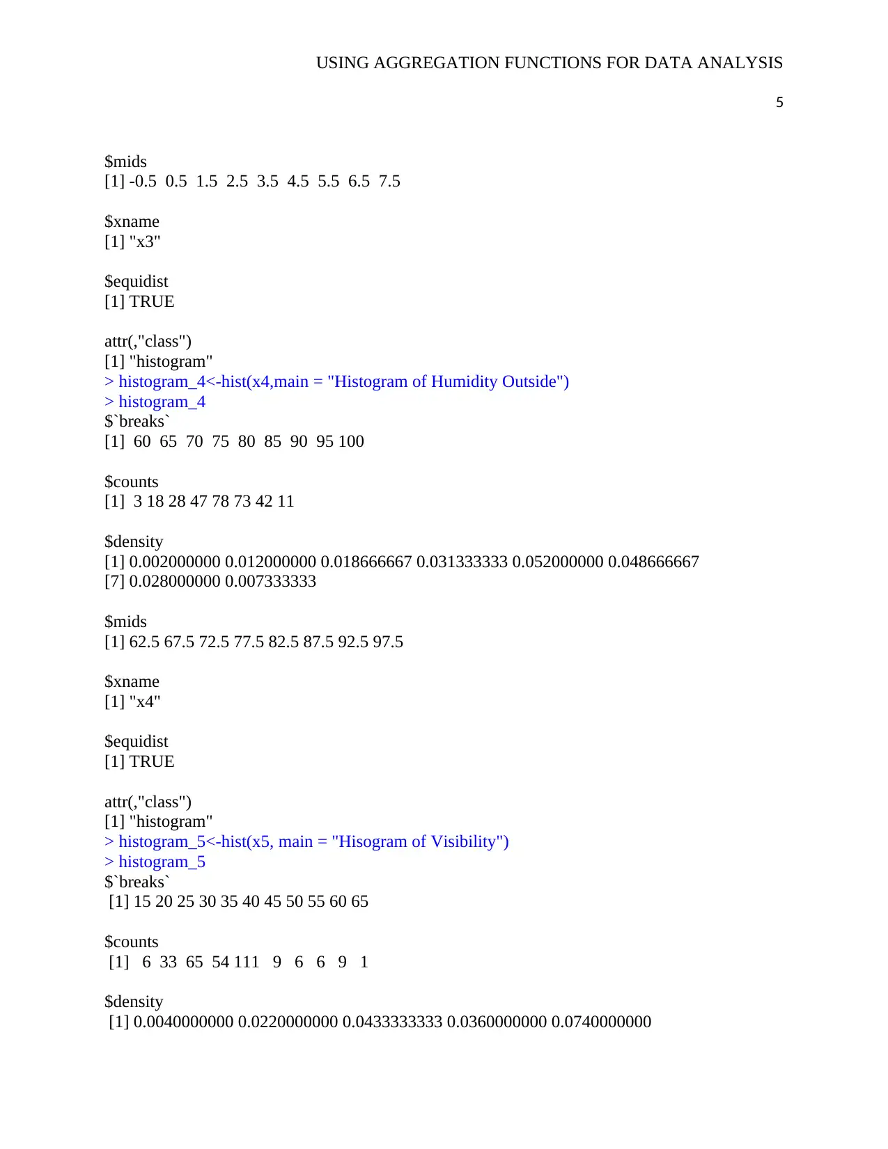
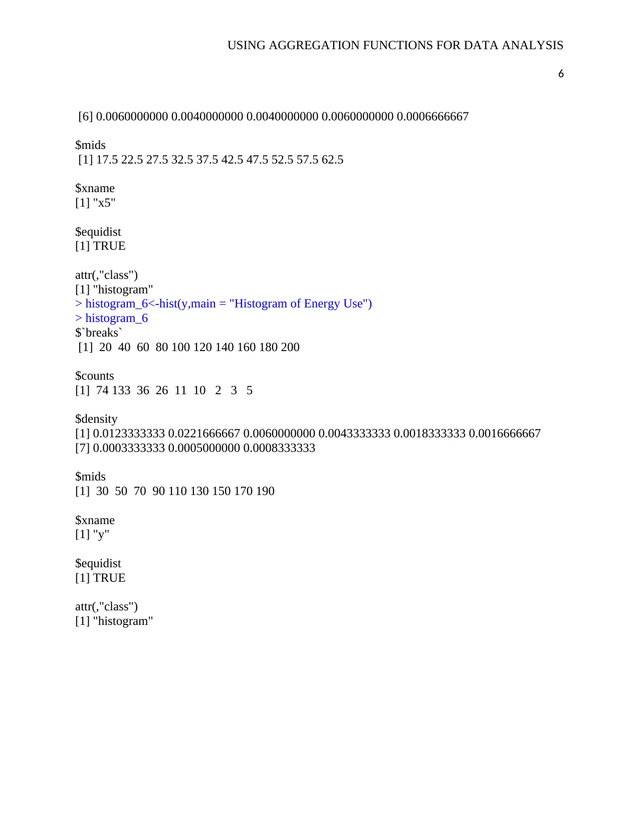
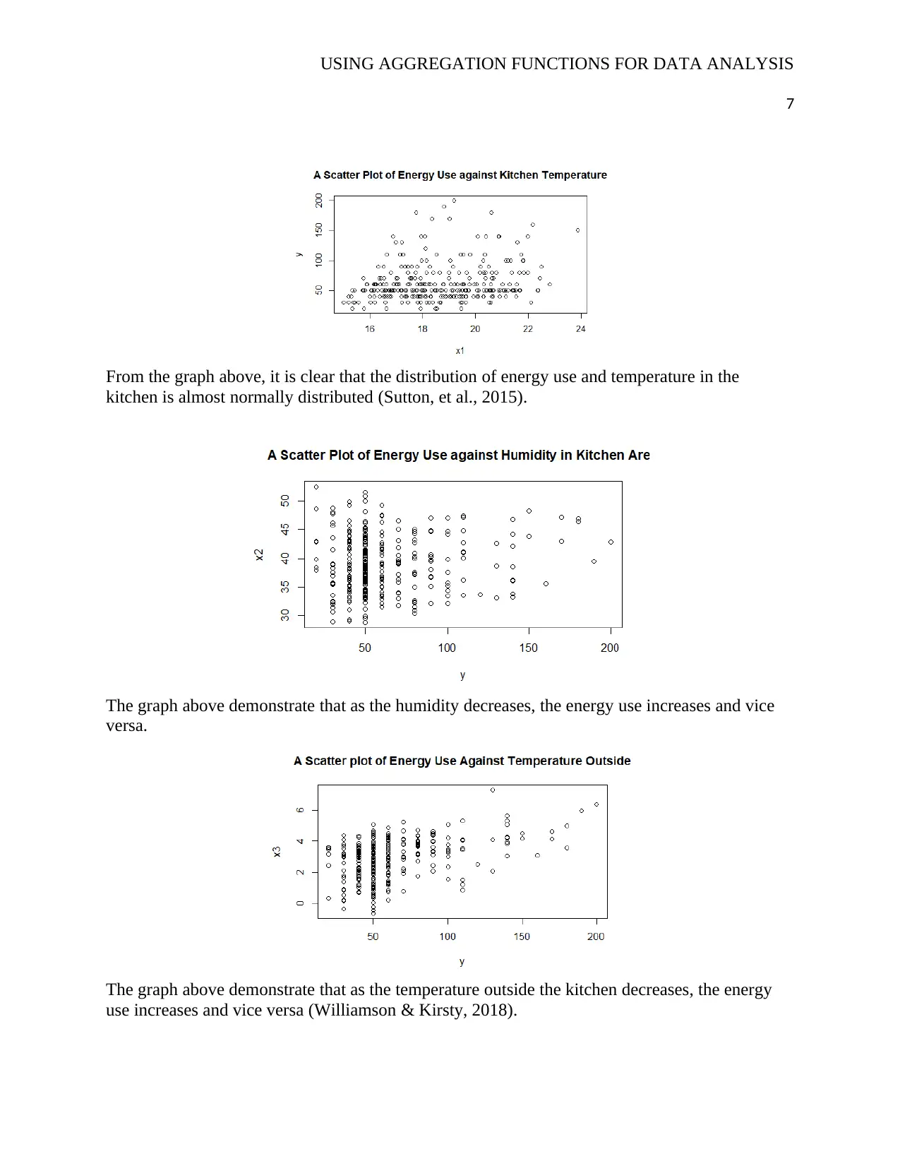
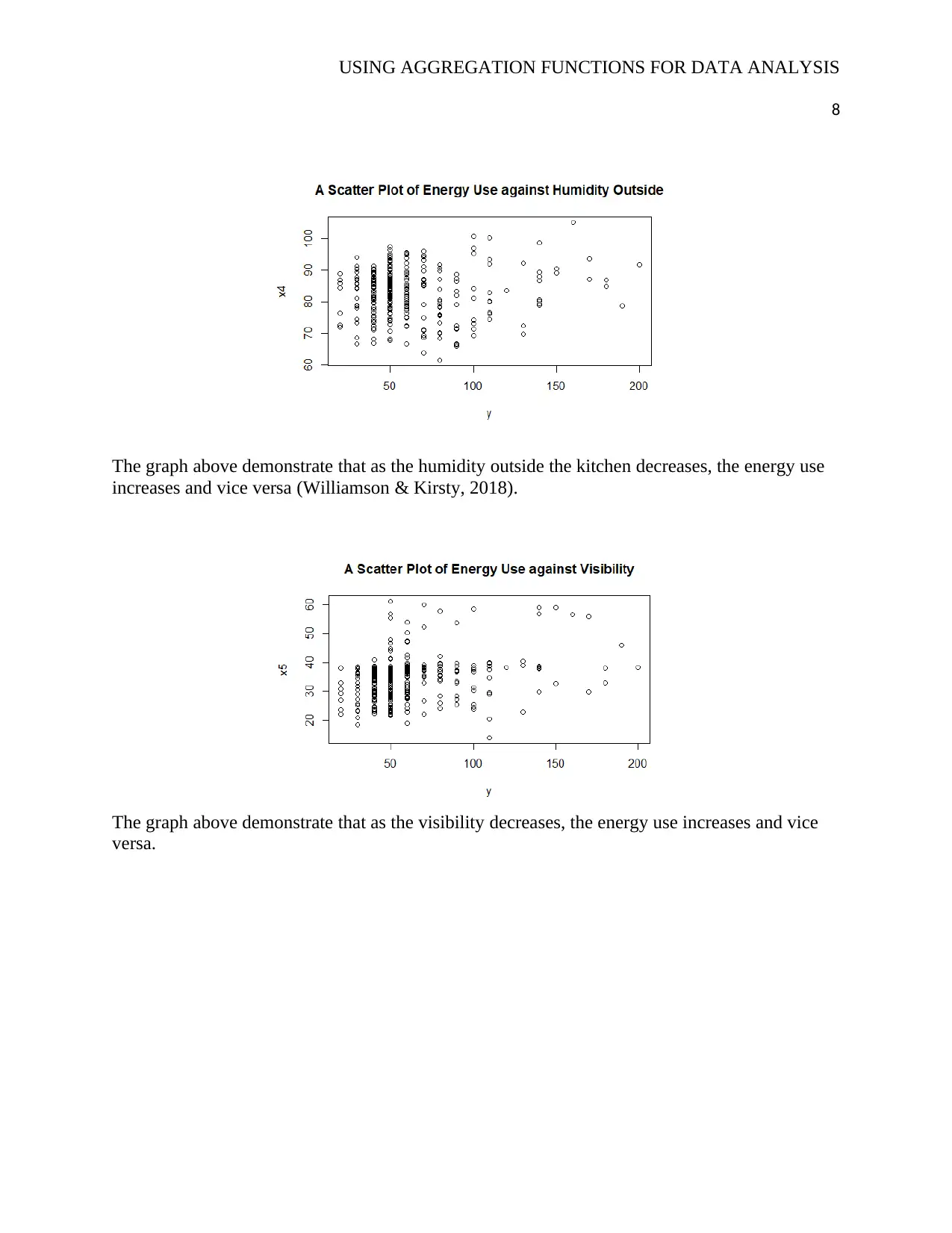
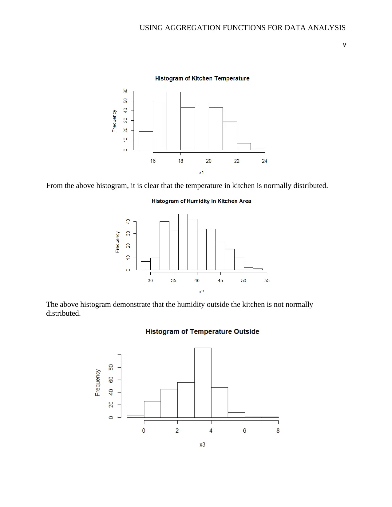
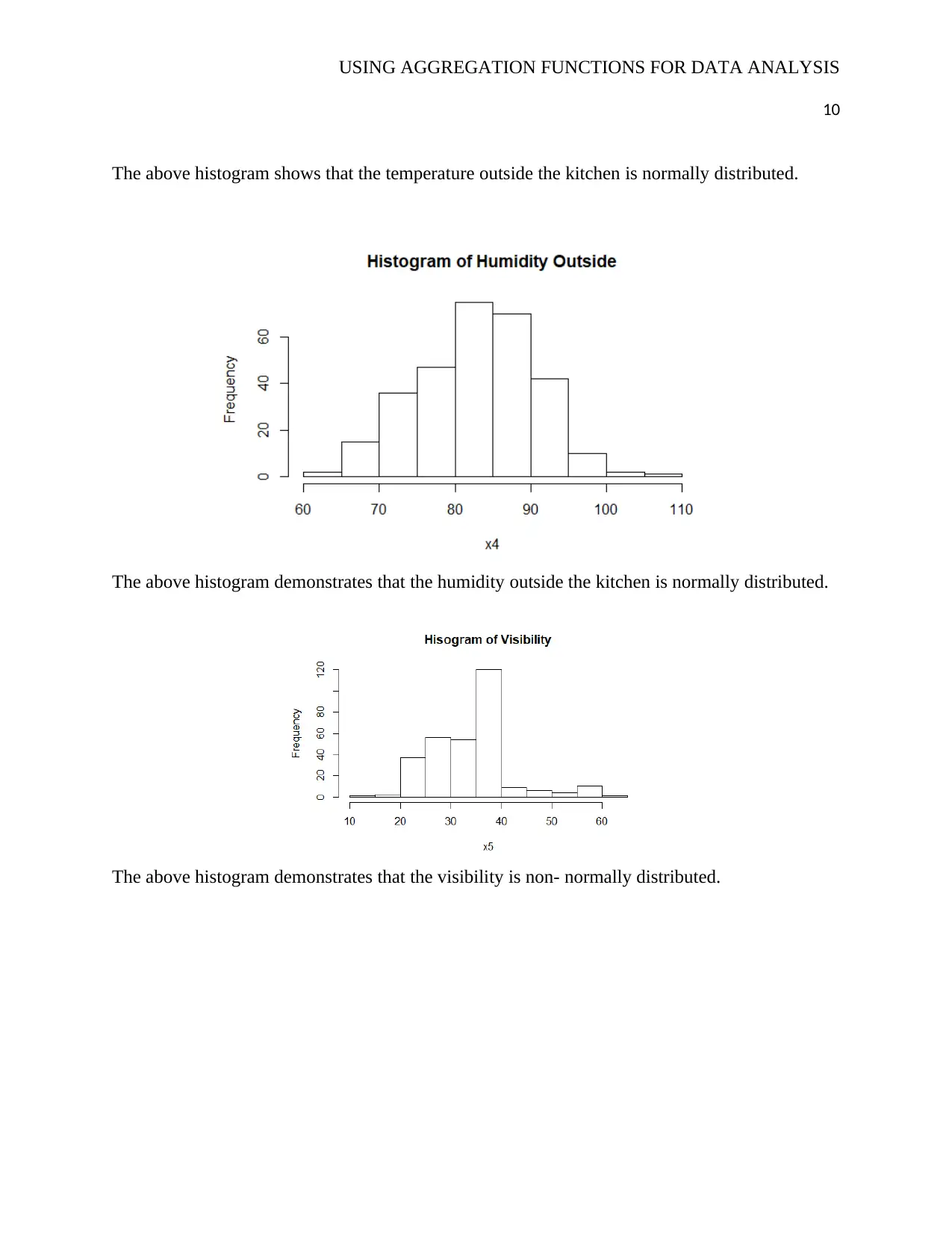
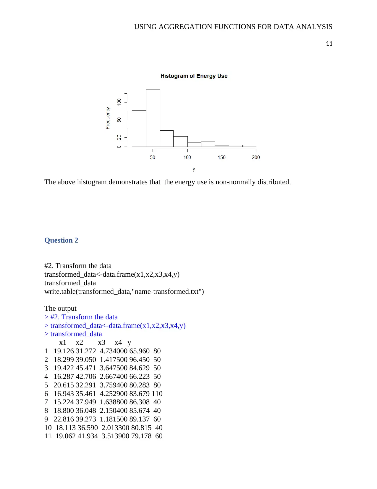
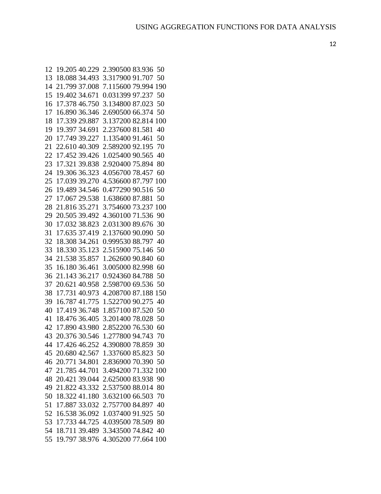
This assignment solution for SIT718 Real World Analytics at Deakin University focuses on data analysis using aggregation functions. The solution begins by importing and preparing the data, which includes energy use of appliances and various environmental factors. It then explores the data through scatter plots and histograms to visualize the relationships between the variables. The solution includes the creation of five scatter plots and six histograms to illustrate the relationships between energy use and variables such as kitchen temperature, humidity, and visibility. The assignment also involves transforming the data and writing it to a text file. The analysis provides insights into how different factors influence energy consumption. The solution demonstrates the use of R programming for data manipulation and visualization to address the assignment's requirements.

USING AGGREGATION FUNCTIONS FOR DATA ANALYSIS
1
USING AGGREGATION FUNCTIONS FOR DATA ANALYSIS
SIT718 Real World Analytics
Assessment Task 3: Problem Solving
Deakin University 1 Future Learn
Name of Student:

USING AGGREGATION FUNCTIONS FOR DATA ANALYSIS
2
Question 1
#1. Understand the data
the.data <- as.matrix(read.table("F:Energy19.txt ")) # (ii)Assigning the data to a matrix
my.data <- the.data[sample(1:671,300),c(1:6)] #(iii) The variable of interest is Energy use of
appliances (Y). To investigate Y, generate a subset of 300 data
data_frame <- data.frame(my.data) #generating a data frame from my.data sample
x1<-data_frame$V1 #extracting X1: Temperature in kitchen area, in Celsius
x2<-data_frame$V2# extracting X2: Humidity in kitchen area, given as a percentage
x3<-data_frame$V3#extracting X3: Temperature outside (from weather station), in Celsius
x4<-data_frame$V4#extracting X4: Humidity outside (from weather station), given as a
percentage
x5<-data_frame$V5#extracting X5: Visibility (from weather station), in km
y<-data_frame$V6#extracting Y: Energy use of appliances, in Wh
#(iv)Using scatter plots and histograms, report on the general relationship betweeneach of the
variables X1, X2, X3, X4, X5 and the variable of interest Y. Include 5scatter plots, 6 histograms,
and 1 or 2 sentences for each of the variables,including the variable of interest Y.
scatter_plot1<-plot(x1,y, main = "A Scatter Plot of Energy Use against Kitchen Temperature")
scatter_plot1
scatter_plot2<-plot(y,x2, main = "A Scatter Plot of Energy Use against Humidity in Kitchen
Area")
scatter_plot2
scatter_plot3<-plot(y,x3,main = "A Scatter plot of Energy Use Against Temperature Outside")
scatter_plot3
scatter_plot4<-plot(y,x4,main = "A Scatter Plot of Energy Use against Humidity Outside")
scatter_plot4
scatter_plot5<-plot(y,x5,main = "A Scatter Plot of Energy Use against Visibility")
scatter_plot5
histogram_1<-hist(x1, main = " Histogram of Kitchen Temperature")
histogram_1
histogram_2<-hist(x2,main = "Histogram of Humidity in Kitchen Area")
histogram_2
histogram_3<-hist(x3,main = "Histogram of Temperature Outside")
histogram_3
histogram_4<-hist(x4,main = "Histogram of Humidity Outside")
histogram_4
histogram_5<-hist(x5, main = "Hisogram of Visibility")
histogram_5
histogram_6<-hist(y,main = "Histogram of Energy Use")
histogram_6
The Output
> #1. Understand the data
> the.data <- as.matrix(read.table("F:Energy19.txt ")) # (ii)Assigning the data to a matrix

USING AGGREGATION FUNCTIONS FOR DATA ANALYSIS
3
> my.data <- the.data[sample(1:671,300),c(1:6)] #(iii) The variable of interest is Energy use of
appliances (Y). To investigate Y, generate a subset of 300 data
> data_frame <- data.frame(my.data) #generating a data frame from my.data sample
> x1<-data_frame$V1 #extracting X1: Temperature in kitchen area, in Celsius
> x2<-data_frame$V2# extracting X2: Humidity in kitchen area, given as a percentage
> x3<-data_frame$V3#extracting X3: Temperature outside (from weather station), in Celsius
> x4<-data_frame$V4#extracting X4: Humidity outside (from weather station), given as a
percentage
> x5<-data_frame$V5#extracting X5: Visibility (from weather station), in km
> y<-data_frame$V6#extracting Y: Energy use of appliances, in Wh
> #(iv)Using scatter plots and histograms, report on the general relationship betweeneach of the
variables X1, X2, X3, X4, X5 and the variable of interest Y. Include 5scatter plots, 6 histograms,
and 1 or 2 sentences for each of the variables,including the variable of interest Y.
> scatter_plot1<-plot(x1,y, main = "A Scatter Plot of Energy Use against Kitchen Temperature")
> scatter_plot1
NULL
> scatter_plot2<-plot(y,x2, main = "A Scatter Plot of Energy Use against Humidity in Kitchen
Area")
> scatter_plot2
NULL
> scatter_plot3<-plot(y,x3,main = "A Scatter plot of Energy Use Against Temperature Outside")
> scatter_plot3
NULL
> scatter_plot4<-plot(y,x4,main = "A Scatter Plot of Energy Use against Humidity Outside")
> scatter_plot4
NULL
> scatter_plot5<-plot(y,x5,main = "A Scatter Plot of Energy Use against Visibility")
> scatter_plot5
NULL
> histogram_1<-hist(x1, main = " Histogram of Kitchen Temperature")
> histogram_1
$`breaks`
[1] 15 16 17 18 19 20 21 22 23 24 25
$counts
[1] 21 43 60 54 48 37 24 10 2 1
$density
[1] 0.070000000 0.143333333 0.200000000 0.180000000 0.160000000 0.123333333
[7] 0.080000000 0.033333333 0.006666667 0.003333333
$mids
[1] 15.5 16.5 17.5 18.5 19.5 20.5 21.5 22.5 23.5 24.5

USING AGGREGATION FUNCTIONS FOR DATA ANALYSIS
4
$xname
[1] "x1"
$equidist
[1] TRUE
attr(,"class")
[1] "histogram"
> histogram_2<-hist(x2,main = "Histogram of Humidity in Kitchen Area")
> histogram_2
$`breaks`
[1] 26 28 30 32 34 36 38 40 42 44 46 48 50 52 54
$counts
[1] 1 8 17 32 31 51 49 40 25 19 16 6 2 3
$density
[1] 0.001666667 0.013333333 0.028333333 0.053333333 0.051666667 0.085000000
[7] 0.081666667 0.066666667 0.041666667 0.031666667 0.026666667 0.010000000
[13] 0.003333333 0.005000000
$mids
[1] 27 29 31 33 35 37 39 41 43 45 47 49 51 53
$xname
[1] "x2"
$equidist
[1] TRUE
attr(,"class")
[1] "histogram"
> histogram_3<-hist(x3,main = "Histogram of Temperature Outside")
> histogram_3
$`breaks`
[1] -1 0 1 2 3 4 5 6 7 8
$counts
[1] 3 22 48 73 91 50 10 2 1
$density
[1] 0.010000000 0.073333333 0.160000000 0.243333333 0.303333333 0.166666667
[7] 0.033333333 0.006666667 0.003333333

USING AGGREGATION FUNCTIONS FOR DATA ANALYSIS
5
$mids
[1] -0.5 0.5 1.5 2.5 3.5 4.5 5.5 6.5 7.5
$xname
[1] "x3"
$equidist
[1] TRUE
attr(,"class")
[1] "histogram"
> histogram_4<-hist(x4,main = "Histogram of Humidity Outside")
> histogram_4
$`breaks`
[1] 60 65 70 75 80 85 90 95 100
$counts
[1] 3 18 28 47 78 73 42 11
$density
[1] 0.002000000 0.012000000 0.018666667 0.031333333 0.052000000 0.048666667
[7] 0.028000000 0.007333333
$mids
[1] 62.5 67.5 72.5 77.5 82.5 87.5 92.5 97.5
$xname
[1] "x4"
$equidist
[1] TRUE
attr(,"class")
[1] "histogram"
> histogram_5<-hist(x5, main = "Hisogram of Visibility")
> histogram_5
$`breaks`
[1] 15 20 25 30 35 40 45 50 55 60 65
$counts
[1] 6 33 65 54 111 9 6 6 9 1
$density
[1] 0.0040000000 0.0220000000 0.0433333333 0.0360000000 0.0740000000

USING AGGREGATION FUNCTIONS FOR DATA ANALYSIS
6
[6] 0.0060000000 0.0040000000 0.0040000000 0.0060000000 0.0006666667
$mids
[1] 17.5 22.5 27.5 32.5 37.5 42.5 47.5 52.5 57.5 62.5
$xname
[1] "x5"
$equidist
[1] TRUE
attr(,"class")
[1] "histogram"
> histogram_6<-hist(y,main = "Histogram of Energy Use")
> histogram_6
$`breaks`
[1] 20 40 60 80 100 120 140 160 180 200
$counts
[1] 74 133 36 26 11 10 2 3 5
$density
[1] 0.0123333333 0.0221666667 0.0060000000 0.0043333333 0.0018333333 0.0016666667
[7] 0.0003333333 0.0005000000 0.0008333333
$mids
[1] 30 50 70 90 110 130 150 170 190
$xname
[1] "y"
$equidist
[1] TRUE
attr(,"class")
[1] "histogram"

USING AGGREGATION FUNCTIONS FOR DATA ANALYSIS
7
From the graph above, it is clear that the distribution of energy use and temperature in the
kitchen is almost normally distributed (Sutton, et al., 2015).
The graph above demonstrate that as the humidity decreases, the energy use increases and vice
versa.
The graph above demonstrate that as the temperature outside the kitchen decreases, the energy
use increases and vice versa (Williamson & Kirsty, 2018).

USING AGGREGATION FUNCTIONS FOR DATA ANALYSIS
8
The graph above demonstrate that as the humidity outside the kitchen decreases, the energy use
increases and vice versa (Williamson & Kirsty, 2018).
The graph above demonstrate that as the visibility decreases, the energy use increases and vice
versa.

USING AGGREGATION FUNCTIONS FOR DATA ANALYSIS
9
From the above histogram, it is clear that the temperature in kitchen is normally distributed.
The above histogram demonstrate that the humidity outside the kitchen is not normally
distributed.

USING AGGREGATION FUNCTIONS FOR DATA ANALYSIS
10
The above histogram shows that the temperature outside the kitchen is normally distributed.
The above histogram demonstrates that the humidity outside the kitchen is normally distributed.
The above histogram demonstrates that the visibility is non- normally distributed.

USING AGGREGATION FUNCTIONS FOR DATA ANALYSIS
11
The above histogram demonstrates that the energy use is non-normally distributed.
Question 2
#2. Transform the data
transformed_data<-data.frame(x1,x2,x3,x4,y)
transformed_data
write.table(transformed_data,"name-transformed.txt")
The output
> #2. Transform the data
> transformed_data<-data.frame(x1,x2,x3,x4,y)
> transformed_data
x1 x2 x3 x4 y
1 19.126 31.272 4.734000 65.960 80
2 18.299 39.050 1.417500 96.450 50
3 19.422 45.471 3.647500 84.629 50
4 16.287 42.706 2.667400 66.223 50
5 20.615 32.291 3.759400 80.283 80
6 16.943 35.461 4.252900 83.679 110
7 15.224 37.949 1.638800 86.308 40
8 18.800 36.048 2.150400 85.674 40
9 22.816 39.273 1.181500 89.137 60
10 18.113 36.590 2.013300 80.815 40
11 19.062 41.934 3.513900 79.178 60

USING AGGREGATION FUNCTIONS FOR DATA ANALYSIS
12
12 19.205 40.229 2.390500 83.936 50
13 18.088 34.493 3.317900 91.707 50
14 21.799 37.008 7.115600 79.994 190
15 19.402 34.671 0.031399 97.237 50
16 17.378 46.750 3.134800 87.023 50
17 16.890 36.346 2.690500 66.374 50
18 17.339 29.887 3.137200 82.814 100
19 19.397 34.691 2.237600 81.581 40
20 17.749 39.227 1.135400 91.461 50
21 22.610 40.309 2.589200 92.195 70
22 17.452 39.426 1.025400 90.565 40
23 17.321 39.838 2.920400 75.894 80
24 19.306 36.323 4.056700 78.457 60
25 17.039 39.270 4.536600 87.797 100
26 19.489 34.546 0.477290 90.516 50
27 17.067 29.538 1.638600 87.881 50
28 21.816 35.271 3.754600 73.237 100
29 20.505 39.492 4.360100 71.536 90
30 17.032 38.823 2.031300 89.676 30
31 17.635 37.419 2.137600 90.090 50
32 18.308 34.261 0.999530 88.797 40
33 18.330 35.123 2.515900 75.146 50
34 21.538 35.857 1.262600 90.840 60
35 16.180 36.461 3.005000 82.998 60
36 21.143 36.217 0.924360 84.788 50
37 20.621 40.958 2.598700 69.536 50
38 17.731 40.973 4.208700 87.188 150
39 16.787 41.775 1.522700 90.275 40
40 17.419 36.748 1.857100 87.520 50
41 18.476 36.405 3.201400 78.028 50
42 17.890 43.980 2.852200 76.530 60
43 20.376 30.546 1.277800 94.743 70
44 17.426 46.252 4.390800 78.859 30
45 20.680 42.567 1.337600 85.823 50
46 20.771 34.801 2.836900 70.390 50
47 21.785 44.701 3.494200 71.332 100
48 20.421 39.044 2.625000 83.938 90
49 21.822 43.332 2.537500 88.014 80
50 18.322 41.180 3.632100 66.503 70
51 17.887 33.032 2.757700 84.897 40
52 16.538 36.092 1.037400 91.925 50
53 17.733 44.725 4.039500 78.509 80
54 18.711 39.489 3.343500 74.842 40
55 19.797 38.976 4.305200 77.664 100