Deakin University SIT718: Linear Programming and Game Theory Project

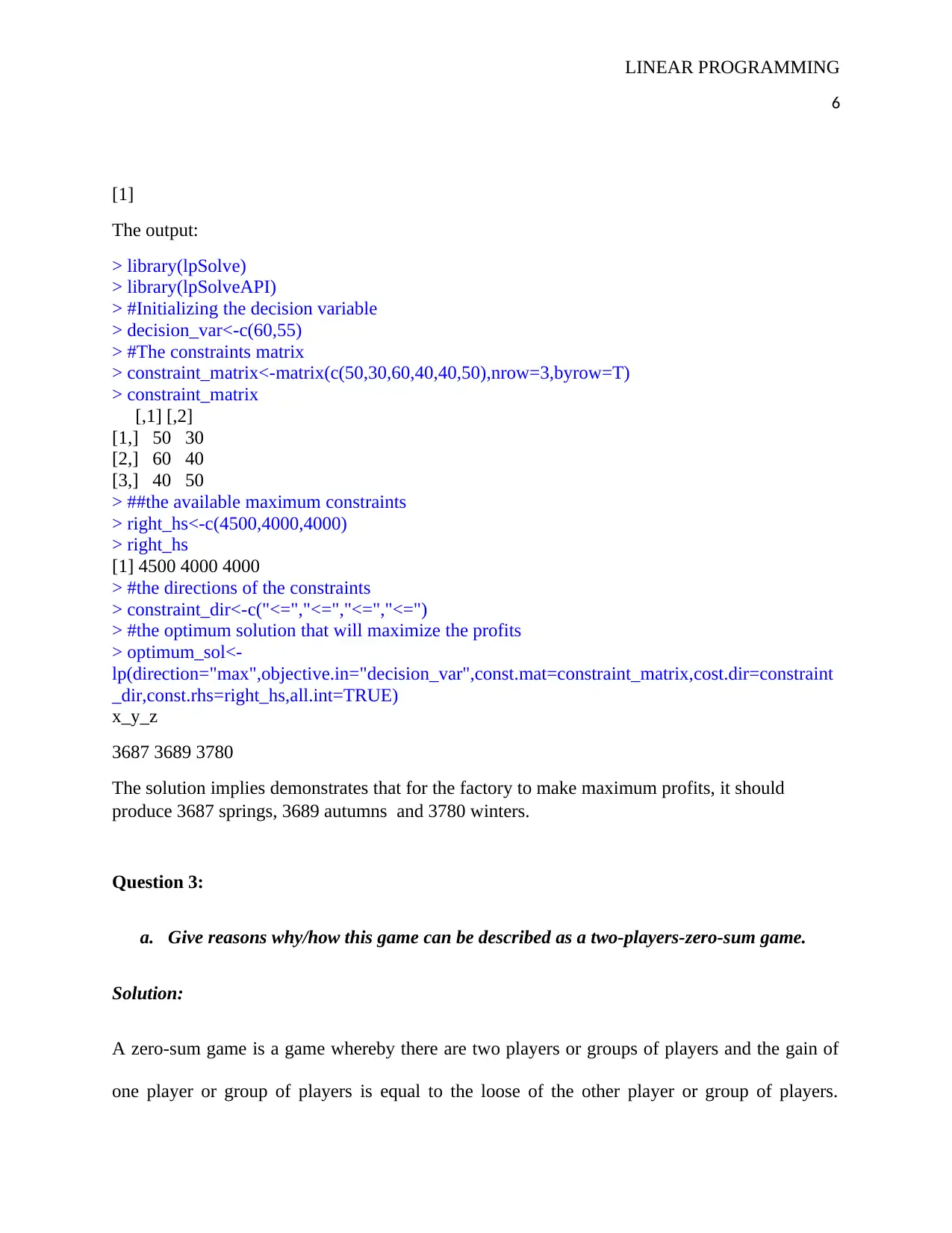
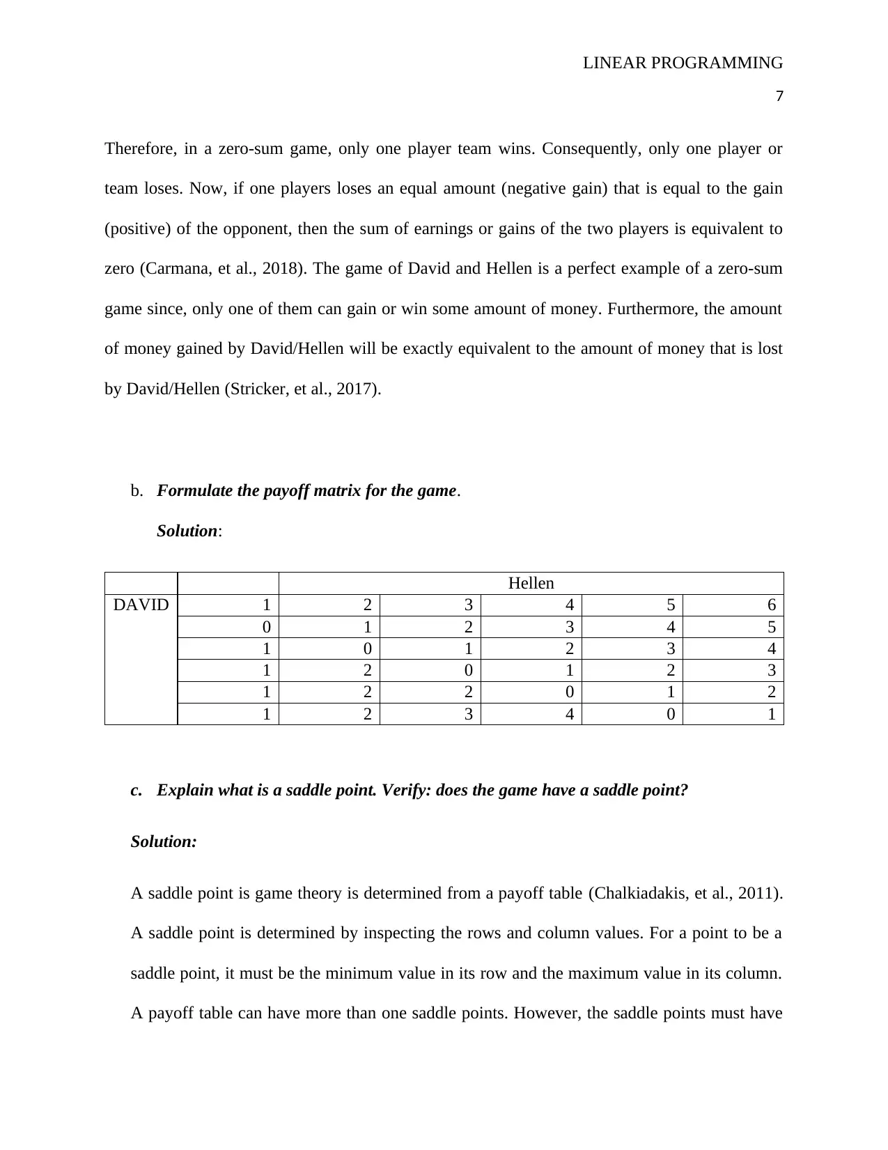
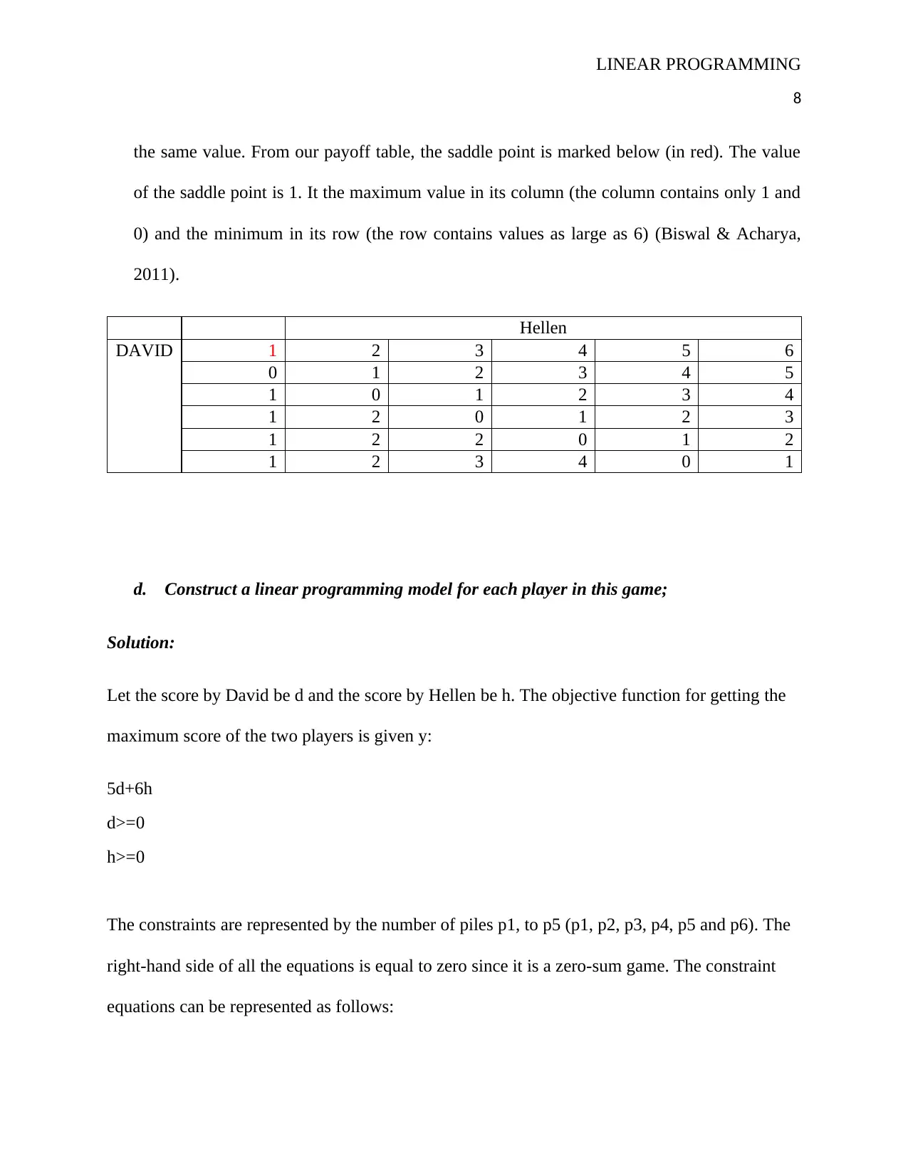
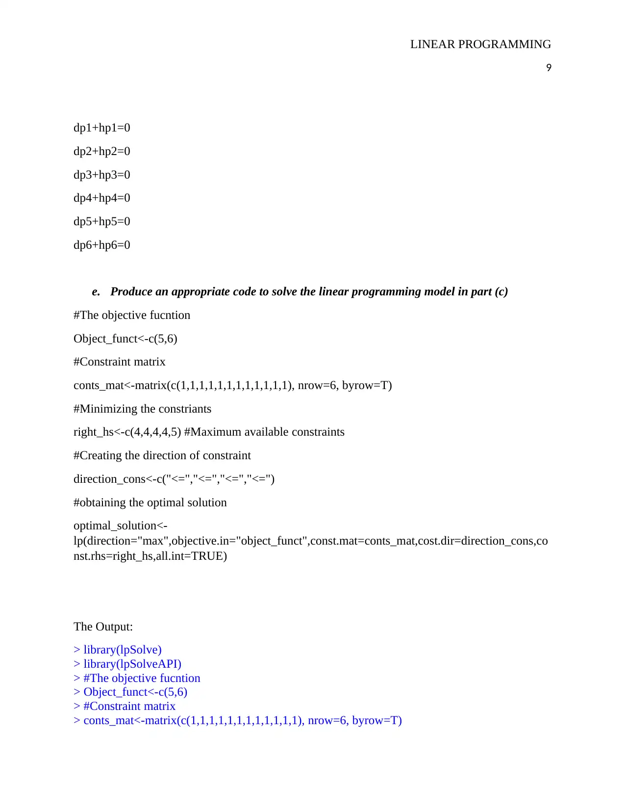
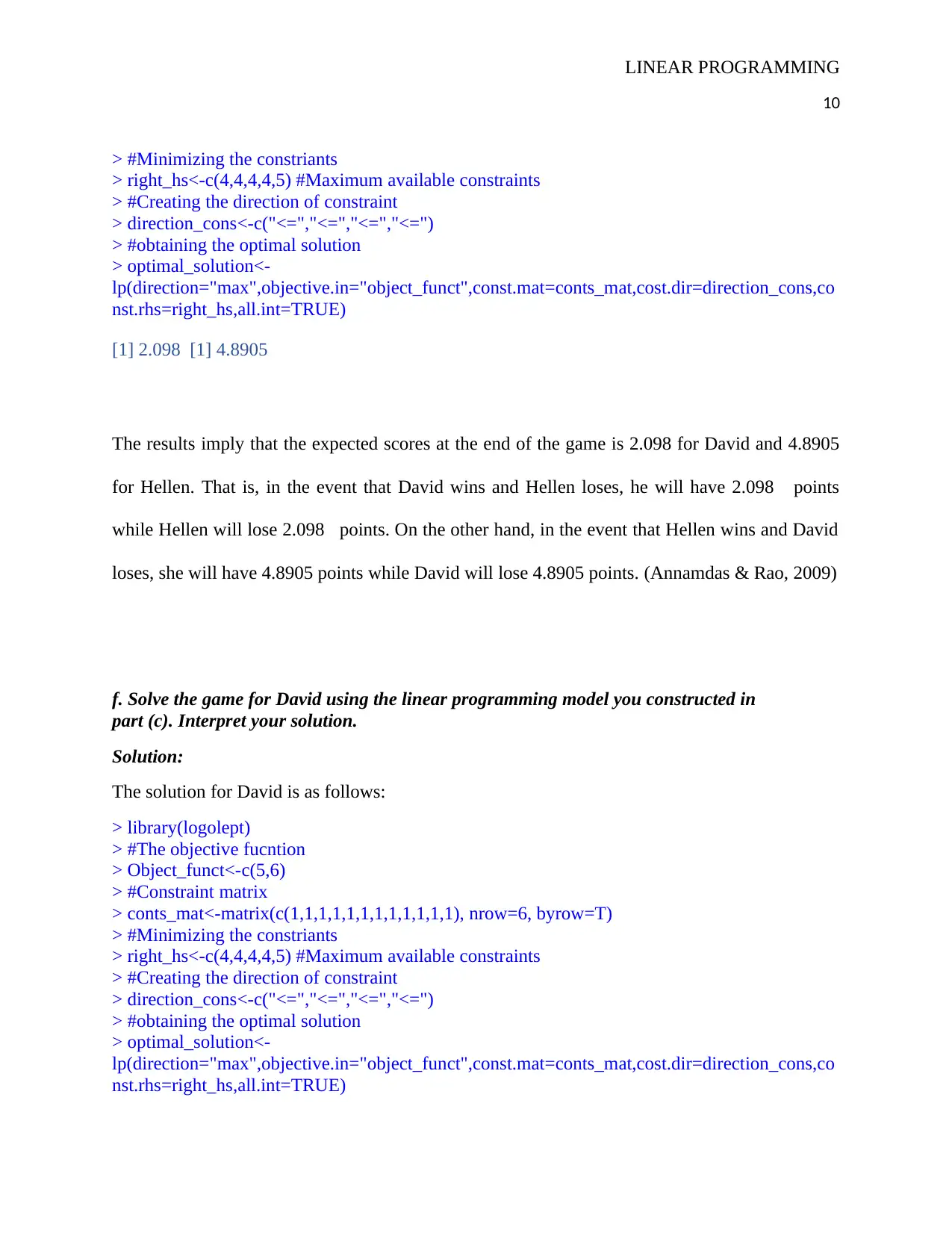
This document presents a comprehensive solution to a real-world analytics assignment focusing on linear programming and game theory. The assignment addresses three key questions: the suitability of linear programming models for optimization, the formulation of linear programming models to maximize profit, and the application of game theory principles to a two-player zero-sum game. The solution includes detailed explanations of linear programming concepts, such as decision variables, constraints, and objective functions, and demonstrates the use of graphical methods and R programming for solving linear programming problems. The assignment also explores game theory, including payoff matrices, saddle points, and the construction of linear programming models for each player. The student provides code to solve the models and interprets the results, illustrating the application of these analytical techniques to real-world scenarios. The references are also included.

LINEAR PROGRAMMING
1
LINEAR PROGRAMMING
Name of student:
Name of Institution:
Date:

LINEAR PROGRAMMING
2
Question one
a. Explain why a linear programming model would be suitable for this case study
Solution:
A linear programming model is a mathematical technique that is used to solve problems that
require the optimization of resources. The optimization can be either minimization or
maximization of the resources (Carmana, et al., 2018). Minimization is done to reduce the cost of
materials or a production process. On the other hand, maximization is done to increase the net
profits by ensuring a proper utilization of the resources that are at hand. The case study in our
scenario is a linear programming model because the aim of the factory is to minimize the cost
producing beverages. The case study has decision variables, the constraint variables and the
objective function. The decision variables are the amounts of mangoes, limes and oranges that
are used in making the beverage. The constraints are the available amounts or units or mangoes,
limes and oranges. The objective function is the cost function (Tamas & Viola, 2011).
b. Formulate a linear programming model
Solution:
A linear programming is formed by stating the objective function, the constraints and the
decision variables. Let beverage A be denoted by A and beverage B denoted by B. Further, let
oranges be denoted by or. Let mangoes be denoted by ma. Let lime be li (Ozdaglar, et al., 2011).
The decision variables:
Lime
Oranges
Mangoes

LINEAR PROGRAMMING
3
Constraints:
or<=4.5
ma<=5
li<=6
4.5or+5ma+6li<=100
The Objective function:
8A+7B
c. Finding the optimum solution by graphical method
Solution:
Lime Orange Mango Cost
A 3 6 4 8
B 8 4 6 7
Constraints A B
Lime 5 6 70
Orange 5 4 70
Mango 5 5 70

LINEAR PROGRAMMING
4
1 2 3
0%
10%
20%
30%
40%
50%
60%
70%
80%
90%
100%
5 6
0
70
0
5 4
0
70
0
5 5
0
70
0
Graphical Solution
Lime Orange Mango
a. Is there a range for the cost ($) of A that can be changed without affecting the
optimum solution obtained above?
Solution:
The range of cost of A cannot be changed since all the constraint variables have a similar value.
Question Two
a. Choose appropriate decision variables, formulate a linear programming model to
determine the optimal product mix that maximizes the profit.
Solution:
The objective of the factory is to maximize the profit, while satisfying the cotton ad wool
proportion constraints. To formulate a linear programming model, the objective function, the
constraints and the decision variables must be determined (Fouad & Hotem, 2010). Let spring be

LINEAR PROGRAMMING
5
denoted by sp, Autumn by at and winter by wt. Also, let cotton be denoted by ct, wool by wl and
silk by sk. The linear programming model is formed as follows:
The objective function:
60sp+55at
sp>=0
at>=0
wt>=0
The following equation outlines the constraints.
50ct+30wl<=4500
60ct+30wl<=4000
40ct+50wl<=4000
b. Find the optimal solution using R/R studio
Solution:
The R code:
#Initializing the decision variable
decision_var<-c(60,55)
#The constraints matrix
constraint_matrix<-matrix(c(50,30,60,40,40,50),nrow=3,byrow=T)
constraint_matrix
##the available maximum constraints
right_hs<-c(4500,4000,4000)
right_hs
#the directions of the constraints
constraint_dir<-c("<=","<=","<=","<=")
#the optimum solution that will maximize the profits
optimum_sol<-
lp(direction="max",objective.in="decision_var",const.mat=constraint_matrix,cost.dir=constraint
_dir,const.rhs=right_hs,all.int=TRUE)

LINEAR PROGRAMMING
6
[1]
The output:
> library(lpSolve)
> library(lpSolveAPI)
> #Initializing the decision variable
> decision_var<-c(60,55)
> #The constraints matrix
> constraint_matrix<-matrix(c(50,30,60,40,40,50),nrow=3,byrow=T)
> constraint_matrix
[,1] [,2]
[1,] 50 30
[2,] 60 40
[3,] 40 50
> ##the available maximum constraints
> right_hs<-c(4500,4000,4000)
> right_hs
[1] 4500 4000 4000
> #the directions of the constraints
> constraint_dir<-c("<=","<=","<=","<=")
> #the optimum solution that will maximize the profits
> optimum_sol<-
lp(direction="max",objective.in="decision_var",const.mat=constraint_matrix,cost.dir=constraint
_dir,const.rhs=right_hs,all.int=TRUE)
x_y_z
3687 3689 3780
The solution implies demonstrates that for the factory to make maximum profits, it should
produce 3687 springs, 3689 autumns and 3780 winters.
Question 3:
a. Give reasons why/how this game can be described as a two-players-zero-sum game.
Solution:
A zero-sum game is a game whereby there are two players or groups of players and the gain of
one player or group of players is equal to the loose of the other player or group of players.

LINEAR PROGRAMMING
7
Therefore, in a zero-sum game, only one player team wins. Consequently, only one player or
team loses. Now, if one players loses an equal amount (negative gain) that is equal to the gain
(positive) of the opponent, then the sum of earnings or gains of the two players is equivalent to
zero (Carmana, et al., 2018). The game of David and Hellen is a perfect example of a zero-sum
game since, only one of them can gain or win some amount of money. Furthermore, the amount
of money gained by David/Hellen will be exactly equivalent to the amount of money that is lost
by David/Hellen (Stricker, et al., 2017).
b. Formulate the payoff matrix for the game.
Solution:
Hellen
DAVID 1 2 3 4 5 6
0 1 2 3 4 5
1 0 1 2 3 4
1 2 0 1 2 3
1 2 2 0 1 2
1 2 3 4 0 1
c. Explain what is a saddle point. Verify: does the game have a saddle point?
Solution:
A saddle point is game theory is determined from a payoff table (Chalkiadakis, et al., 2011).
A saddle point is determined by inspecting the rows and column values. For a point to be a
saddle point, it must be the minimum value in its row and the maximum value in its column.
A payoff table can have more than one saddle points. However, the saddle points must have

LINEAR PROGRAMMING
8
the same value. From our payoff table, the saddle point is marked below (in red). The value
of the saddle point is 1. It the maximum value in its column (the column contains only 1 and
0) and the minimum in its row (the row contains values as large as 6) (Biswal & Acharya,
2011).
Hellen
DAVID 1 2 3 4 5 6
0 1 2 3 4 5
1 0 1 2 3 4
1 2 0 1 2 3
1 2 2 0 1 2
1 2 3 4 0 1
d. Construct a linear programming model for each player in this game;
Solution:
Let the score by David be d and the score by Hellen be h. The objective function for getting the
maximum score of the two players is given y:
5d+6h
d>=0
h>=0
The constraints are represented by the number of piles p1, to p5 (p1, p2, p3, p4, p5 and p6). The
right-hand side of all the equations is equal to zero since it is a zero-sum game. The constraint
equations can be represented as follows:

LINEAR PROGRAMMING
9
dp1+hp1=0
dp2+hp2=0
dp3+hp3=0
dp4+hp4=0
dp5+hp5=0
dp6+hp6=0
e. Produce an appropriate code to solve the linear programming model in part (c)
#The objective fucntion
Object_funct<-c(5,6)
#Constraint matrix
conts_mat<-matrix(c(1,1,1,1,1,1,1,1,1,1,1,1), nrow=6, byrow=T)
#Minimizing the constriants
right_hs<-c(4,4,4,4,5) #Maximum available constraints
#Creating the direction of constraint
direction_cons<-c("<=","<=","<=","<=")
#obtaining the optimal solution
optimal_solution<-
lp(direction="max",objective.in="object_funct",const.mat=conts_mat,cost.dir=direction_cons,co
nst.rhs=right_hs,all.int=TRUE)
The Output:
> library(lpSolve)
> library(lpSolveAPI)
> #The objective fucntion
> Object_funct<-c(5,6)
> #Constraint matrix
> conts_mat<-matrix(c(1,1,1,1,1,1,1,1,1,1,1,1), nrow=6, byrow=T)

LINEAR PROGRAMMING
10
> #Minimizing the constriants
> right_hs<-c(4,4,4,4,5) #Maximum available constraints
> #Creating the direction of constraint
> direction_cons<-c("<=","<=","<=","<=")
> #obtaining the optimal solution
> optimal_solution<-
lp(direction="max",objective.in="object_funct",const.mat=conts_mat,cost.dir=direction_cons,co
nst.rhs=right_hs,all.int=TRUE)
[1] 2.098 [1] 4.8905
The results imply that the expected scores at the end of the game is 2.098 for David and 4.8905
for Hellen. That is, in the event that David wins and Hellen loses, he will have 2.098 points
while Hellen will lose 2.098 points. On the other hand, in the event that Hellen wins and David
loses, she will have 4.8905 points while David will lose 4.8905 points. (Annamdas & Rao, 2009)
f. Solve the game for David using the linear programming model you constructed in
part (c). Interpret your solution.
Solution:
The solution for David is as follows:
> library(logolept)
> #The objective fucntion
> Object_funct<-c(5,6)
> #Constraint matrix
> conts_mat<-matrix(c(1,1,1,1,1,1,1,1,1,1,1,1), nrow=6, byrow=T)
> #Minimizing the constriants
> right_hs<-c(4,4,4,4,5) #Maximum available constraints
> #Creating the direction of constraint
> direction_cons<-c("<=","<=","<=","<=")
> #obtaining the optimal solution
> optimal_solution<-
lp(direction="max",objective.in="object_funct",const.mat=conts_mat,cost.dir=direction_cons,co
nst.rhs=right_hs,all.int=TRUE)

LINEAR PROGRAMMING
11
[1] 2.098
The solution implies that if David wins, then his total score will be 2.098. since this is a zero-
sum game, the Hellen will lose the 2.098 in the game in the event that David wins (Stricker, et
al., 2017).

LINEAR PROGRAMMING
12
References
Annamdas, K. K. & Rao, S. S., 2009. Multi-objective optimization of engineering systems using
game theory and particle swarm optimization. The Journal of Engineering Optimization, 41(08),
pp. 23-28.
Biswal, M. P. & Acharya, S., 2011. Solving multi-choice linear programming problems by
interpolating polynomials. Mathematical and Computer Modelling, 54(5), pp. 12-15.
Carmana, Rane, Delarue & Francois, 2018. Probabilistic Theory of Mean Field Games with
Applications I. The Journal of Probability Theory and Stochastic Modelling, 83(10), pp. 12-18.
Chalkiadakis, et al., 2011. Computational Aspects of Cooperative Game Theory. Synthesis
Lectures on Artificial Intelligence and Machine Learning, 5(6), pp. 1-8.
Fouad, B. A. & Hotem, M., 2010. A compromise solution for the multiobjective stochastic linear
programming under partial uncertainty. European Journal of Operational Research, 202(01), pp.
2-11.
Ozdaglar, Asuman, Menache & Ishai, 2011. Network Games: Theory, Models, and Dynamics.
Synthesis Lectures on Communication Networks, 04(01), pp. 22-27.
Stricker, et al., 2017. Selecting key performance indicators for production with a linear
programming approach. International Journal of Production Research, 02(1), pp. 21-26.
Tamas, K. & Viola, T., 2011. A practical approach to sensitivity analysis in linear programming
under degeneracy for management decision making. International Journal of Production
Economics, 131(01), pp. 2-21.