DecaSport Project: Financial Analysis, Capital Structure, and WACC
VerifiedAdded on 2023/04/23
|18
|3830
|62
Report
AI Summary
This report presents a comprehensive financial analysis of DecaSport's new sport shoe project, evaluating its financial viability through various metrics. The analysis includes the calculation of Net Present Value (NPV), payback period, and profitability index under base, best-case, and worst-case scenarios. It also examines the company's capital structure, focusing on the weighted average cost of capital (WACC) and comparing it with a competitor, Common Wealth Bank. The report further discusses different payment options for the new production machines, recommending the quarterly payment option based on the lowest net payment. Additionally, it assesses ANZ Bank's capital structure, financial performance, and liquidity position, highlighting improvements in profitability and liquidity coverage.

Assessment 3
1
1
Paraphrase This Document
Need a fresh take? Get an instant paraphrase of this document with our AI Paraphraser
Part-A
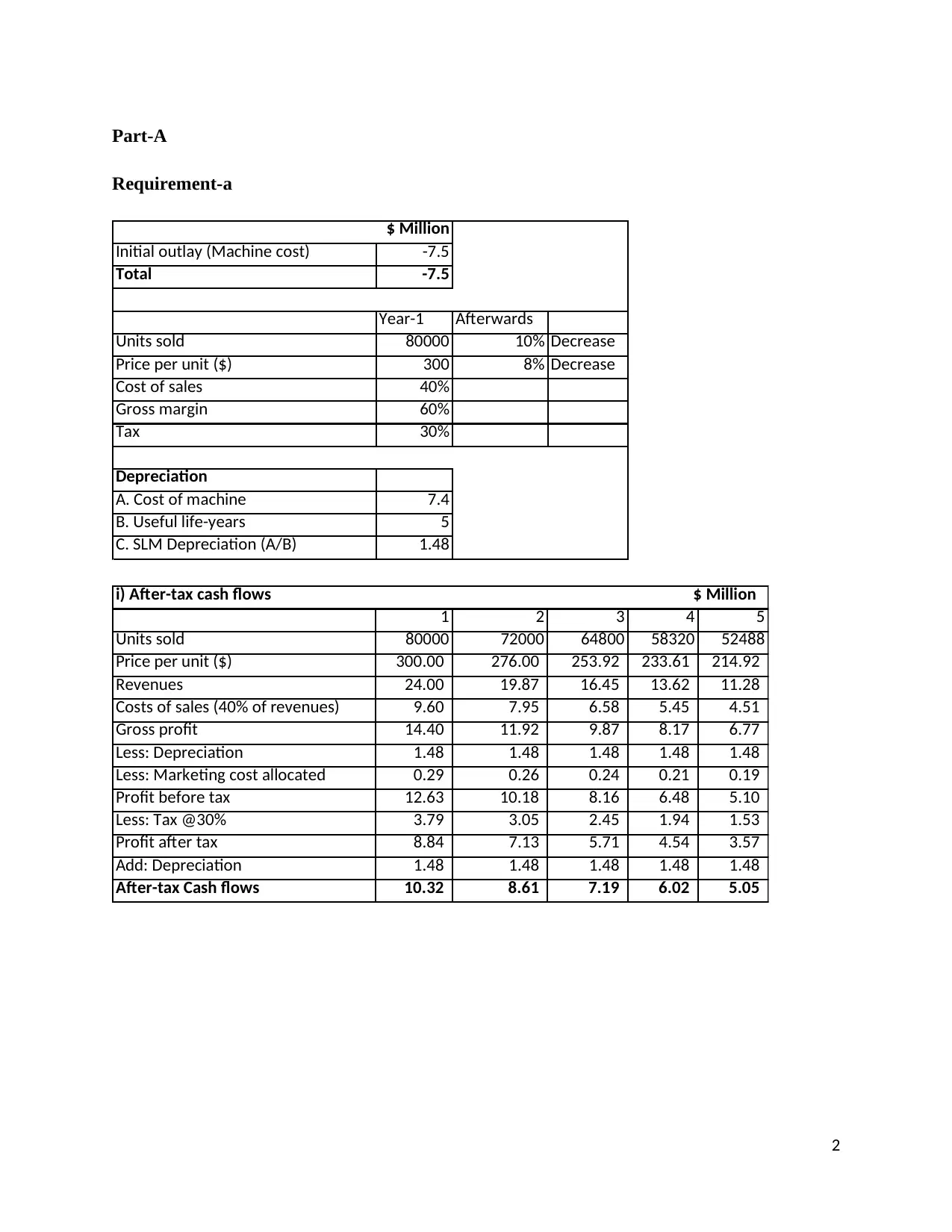
Requirement-a
$ Million
Initial outlay (Machine cost) -7.5
Total -7.5
Year-1 Afterwards
Units sold 80000 10% Decrease
Price per unit ($) 300 8% Decrease
Cost of sales 40%
Gross margin 60%
Tax 30%
Depreciation
A. Cost of machine 7.4
B. Useful life-years 5
C. SLM Depreciation (A/B) 1.48
1 2 3 4 5
Units sold 80000 72000 64800 58320 52488
Price per unit ($) 300.00 276.00 253.92 233.61 214.92
Revenues 24.00 19.87 16.45 13.62 11.28
Costs of sales (40% of revenues) 9.60 7.95 6.58 5.45 4.51
Gross profit 14.40 11.92 9.87 8.17 6.77
Less: Depreciation 1.48 1.48 1.48 1.48 1.48
Less: Marketing cost allocated 0.29 0.26 0.24 0.21 0.19
Profit before tax 12.63 10.18 8.16 6.48 5.10
Less: Tax @30% 3.79 3.05 2.45 1.94 1.53
Profit after tax 8.84 7.13 5.71 4.54 3.57
Add: Depreciation 1.48 1.48 1.48 1.48 1.48
After-tax Cash flows 10.32 8.61 7.19 6.02 5.05
i) After-tax cash flows $ Million
2
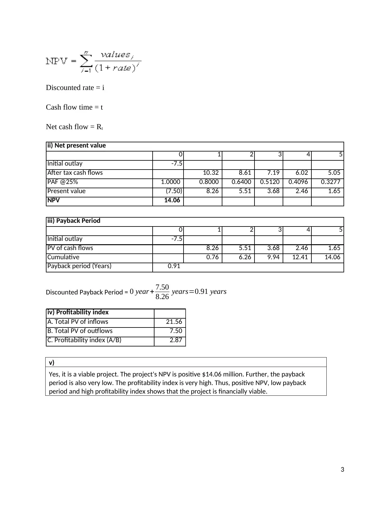
Discounted rate = i
Cash flow time = t
Net cash flow = Rt
0 1 2 3 4 5
Initial outlay -7.5
After tax cash flows 10.32 8.61 7.19 6.02 5.05
PAF @25% 1.0000 0.8000 0.6400 0.5120 0.4096 0.3277
Present value (7.50) 8.26 5.51 3.68 2.46 1.65
NPV 14.06
ii) Net present value
0 1 2 3 4 5
Initial outlay -7.5
PV of cash flows 8.26 5.51 3.68 2.46 1.65
Cumulative 0.76 6.26 9.94 12.41 14.06
Payback period (Years) 0.91
iii) Payback Period
Discounted Payback Period = 0 year+ 7.50
8.26 years=0.91 years
iv) Profitability index
A. Total PV of inflows 21.56
B. Total PV of outflows 7.50
C. Profitability index (A/B) 2.87
v)
Yes, it is a viable project. The project's NPV is positive $14.06 million. Further, the payback
period is also very low. The profitability index is very high. Thus, positive NPV, low payback
period and high profitability index shows that the project is financially viable.
3
⊘ This is a preview!⊘
Do you want full access?
Subscribe today to unlock all pages.
Trusted by 1+ million students worldwide
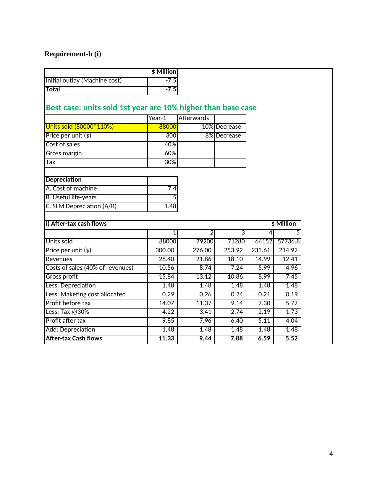
Requirement-b (i)
$ Million
Initial outlay (Machine cost) -7.5
Total -7.5
Best case: units sold 1st year are 10% higher than base case
Year-1 Afterwards
Units sold (80000*110%) 88000 10% Decrease
Price per unit ($) 300 8% Decrease
Cost of sales 40%
Gross margin 60%
Tax 30%
Depreciation
A. Cost of machine 7.4
B. Useful life-years 5
C. SLM Depreciation (A/B) 1.48
1 2 3 4 5
Units sold 88000 79200 71280 64152 57736.8
Price per unit ($) 300.00 276.00 253.92 233.61 214.92
Revenues 26.40 21.86 18.10 14.99 12.41
Costs of sales (40% of revenues) 10.56 8.74 7.24 5.99 4.96
Gross profit 15.84 13.12 10.86 8.99 7.45
Less: Depreciation 1.48 1.48 1.48 1.48 1.48
Less: Maketing cost allocated 0.29 0.26 0.24 0.21 0.19
Profit before tax 14.07 11.37 9.14 7.30 5.77
Less: Tax @30% 4.22 3.41 2.74 2.19 1.73
Profit after tax 9.85 7.96 6.40 5.11 4.04
Add: Depreciation 1.48 1.48 1.48 1.48 1.48
After-tax Cash flows 11.33 9.44 7.88 6.59 5.52
i) After-tax cash flows $ Million
4
Paraphrase This Document
Need a fresh take? Get an instant paraphrase of this document with our AI Paraphraser
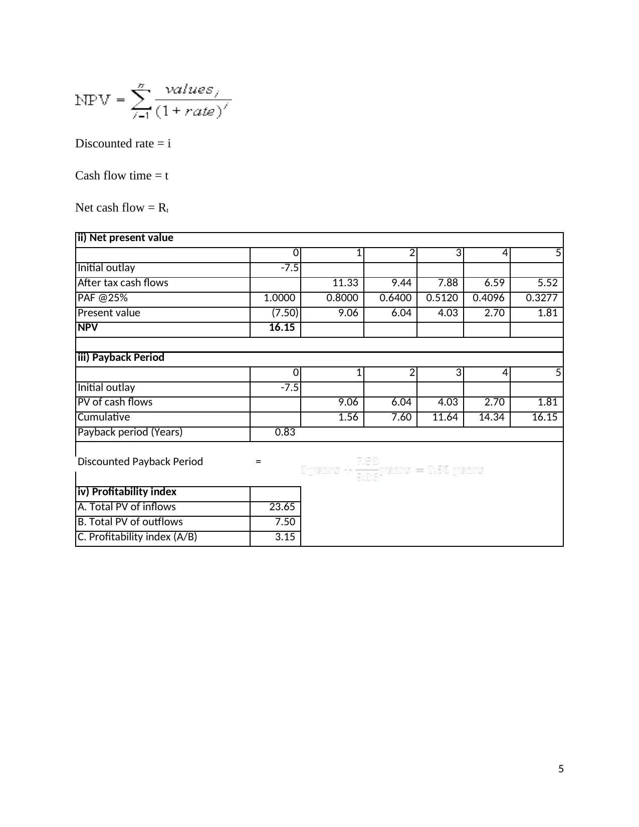
Discounted rate = i
Cash flow time = t
Net cash flow = Rt
0 1 2 3 4 5
Initial outlay -7.5
After tax cash flows 11.33 9.44 7.88 6.59 5.52
PAF @25% 1.0000 0.8000 0.6400 0.5120 0.4096 0.3277
Present value (7.50) 9.06 6.04 4.03 2.70 1.81
NPV 16.15
0 1 2 3 4 5
Initial outlay -7.5
PV of cash flows 9.06 6.04 4.03 2.70 1.81
Cumulative 1.56 7.60 11.64 14.34 16.15
Payback period (Years) 0.83
Discounted Payback Period =
iv) Profitability index
A. Total PV of inflows 23.65
B. Total PV of outflows 7.50
C. Profitability index (A/B) 3.15
ii) Net present value
iii) Payback Period
5
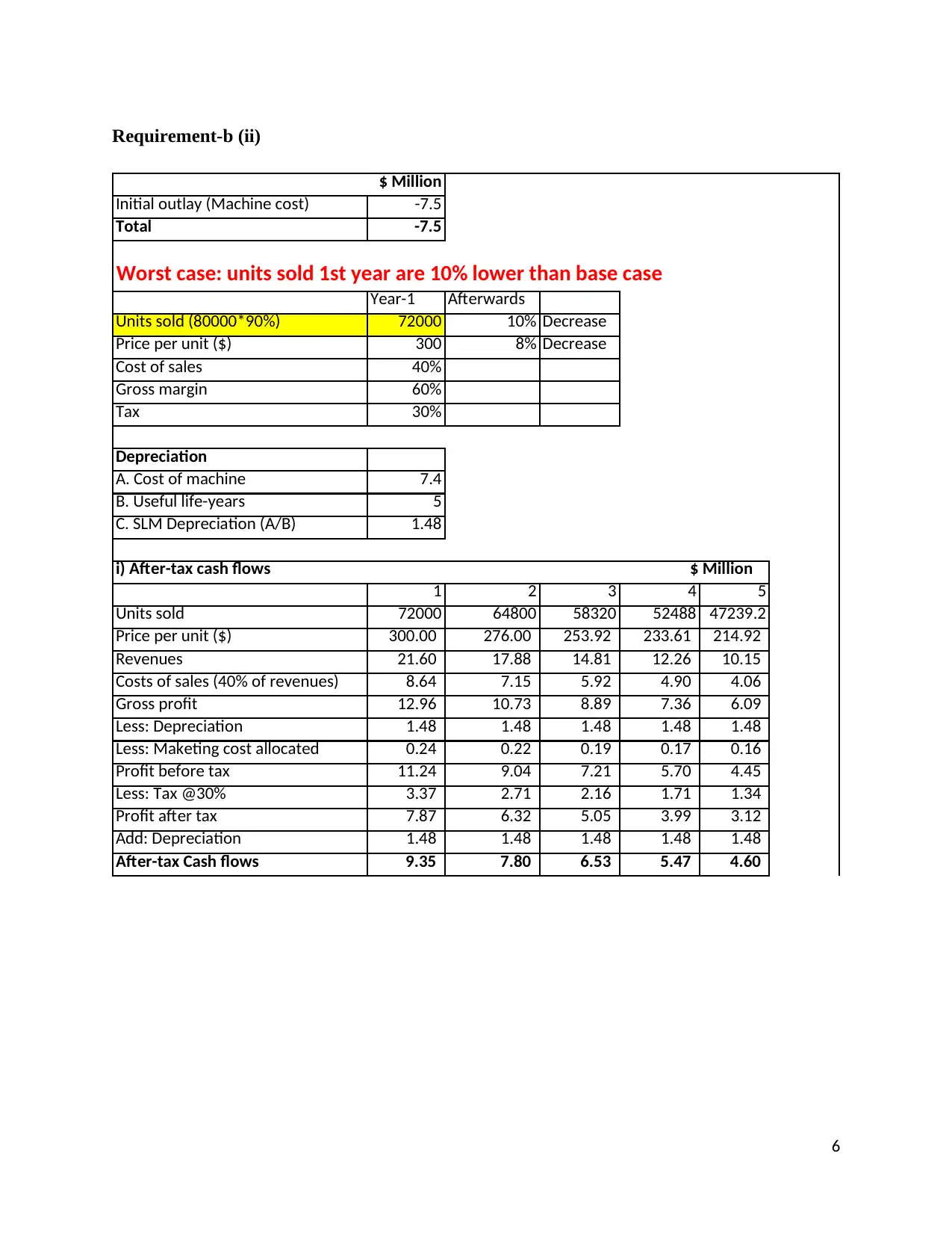
Requirement-b (ii)
$ Million
Initial outlay (Machine cost) -7.5
Total -7.5
Worst case: units sold 1st year are 10% lower than base case
Year-1 Afterwards
Units sold (80000*90%) 72000 10% Decrease
Price per unit ($) 300 8% Decrease
Cost of sales 40%
Gross margin 60%
Tax 30%
Depreciation
A. Cost of machine 7.4
B. Useful life-years 5
C. SLM Depreciation (A/B) 1.48
1 2 3 4 5
Units sold 72000 64800 58320 52488 47239.2
Price per unit ($) 300.00 276.00 253.92 233.61 214.92
Revenues 21.60 17.88 14.81 12.26 10.15
Costs of sales (40% of revenues) 8.64 7.15 5.92 4.90 4.06
Gross profit 12.96 10.73 8.89 7.36 6.09
Less: Depreciation 1.48 1.48 1.48 1.48 1.48
Less: Maketing cost allocated 0.24 0.22 0.19 0.17 0.16
Profit before tax 11.24 9.04 7.21 5.70 4.45
Less: Tax @30% 3.37 2.71 2.16 1.71 1.34
Profit after tax 7.87 6.32 5.05 3.99 3.12
Add: Depreciation 1.48 1.48 1.48 1.48 1.48
After-tax Cash flows 9.35 7.80 6.53 5.47 4.60
i) After-tax cash flows $ Million
6
⊘ This is a preview!⊘
Do you want full access?
Subscribe today to unlock all pages.
Trusted by 1+ million students worldwide
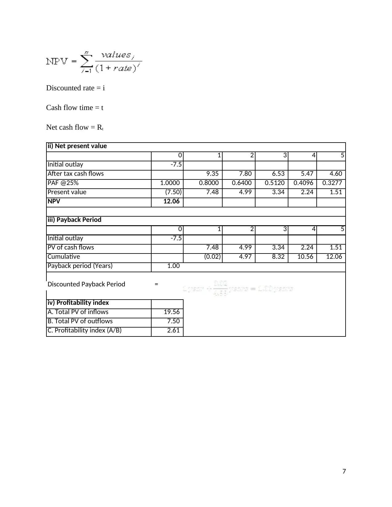
Discounted rate = i
Cash flow time = t
Net cash flow = Rt
0 1 2 3 4 5
Initial outlay -7.5
After tax cash flows 9.35 7.80 6.53 5.47 4.60
PAF @25% 1.0000 0.8000 0.6400 0.5120 0.4096 0.3277
Present value (7.50) 7.48 4.99 3.34 2.24 1.51
NPV 12.06
0 1 2 3 4 5
Initial outlay -7.5
PV of cash flows 7.48 4.99 3.34 2.24 1.51
Cumulative (0.02) 4.97 8.32 10.56 12.06
Payback period (Years) 1.00
Discounted Payback Period =
iv) Profitability index
A. Total PV of inflows 19.56
B. Total PV of outflows 7.50
C. Profitability index (A/B) 2.61
ii) Net present value
iii) Payback Period
7
Paraphrase This Document
Need a fresh take? Get an instant paraphrase of this document with our AI Paraphraser
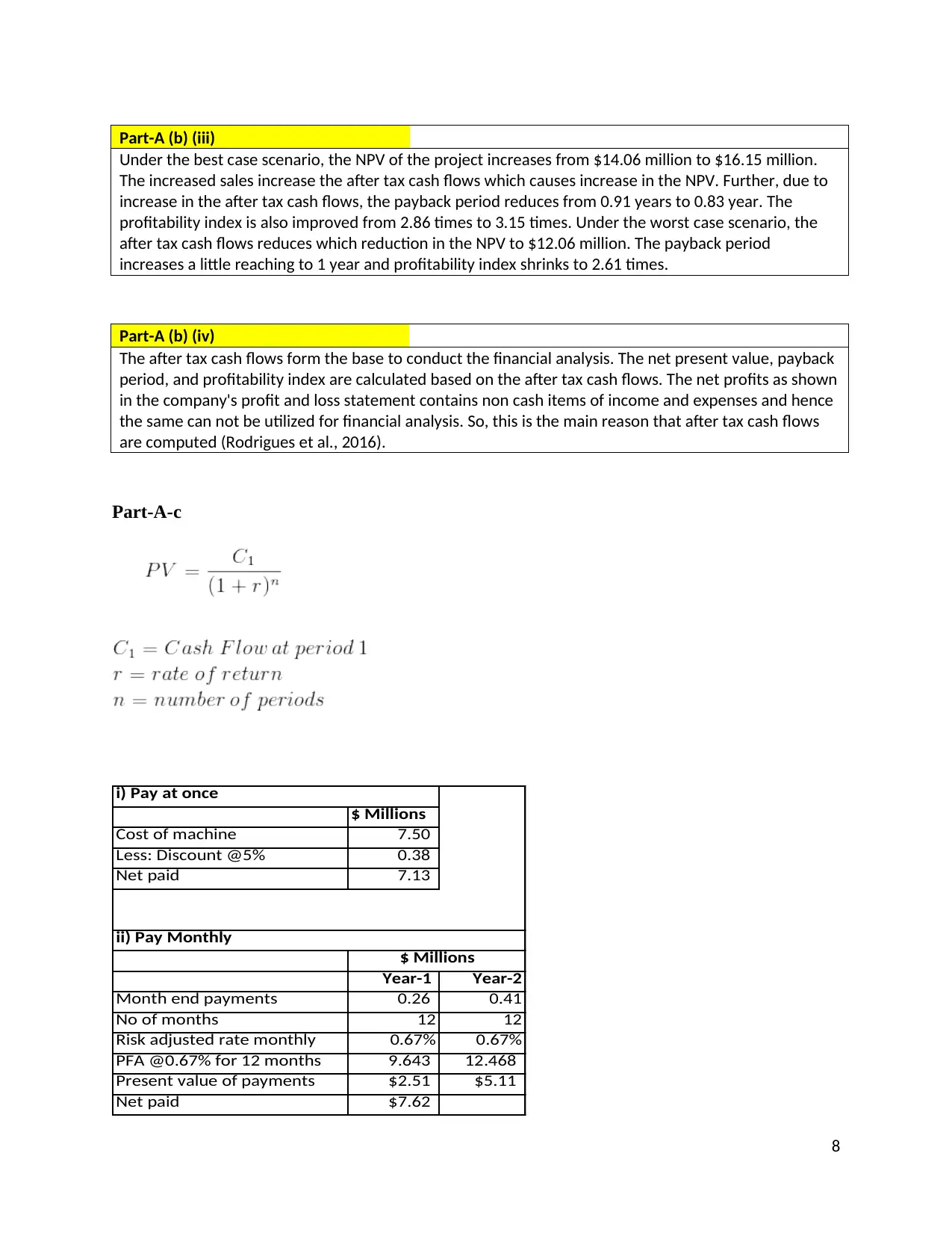
Part-A (b) (iii)
Under the best case scenario, the NPV of the project increases from $14.06 million to $16.15 million.
The increased sales increase the after tax cash flows which causes increase in the NPV. Further, due to
increase in the after tax cash flows, the payback period reduces from 0.91 years to 0.83 year. The
profitability index is also improved from 2.86 times to 3.15 times. Under the worst case scenario, the
after tax cash flows reduces which reduction in the NPV to $12.06 million. The payback period
increases a little reaching to 1 year and profitability index shrinks to 2.61 times.
Part-A (b) (iv)
The after tax cash flows form the base to conduct the financial analysis. The net present value, payback
period, and profitability index are calculated based on the after tax cash flows. The net profits as shown
in the company's profit and loss statement contains non cash items of income and expenses and hence
the same can not be utilized for financial analysis. So, this is the main reason that after tax cash flows
are computed (Rodrigues et al., 2016).
Part-A-c
$ Millions
Cost of machine 7.50
Less: Discount @5% 0.38
Net paid 7.13
Year-1 Year-2
Month end payments 0.26 0.41
No of months 12 12
Risk adjusted rate monthly 0.67% 0.67%
PFA @0.67% for 12 months 9.643 12.468
Present value of payments $2.51 $5.11
Net paid $7.62
i) Pay at once
$ Millions
ii) Pay Monthly
8
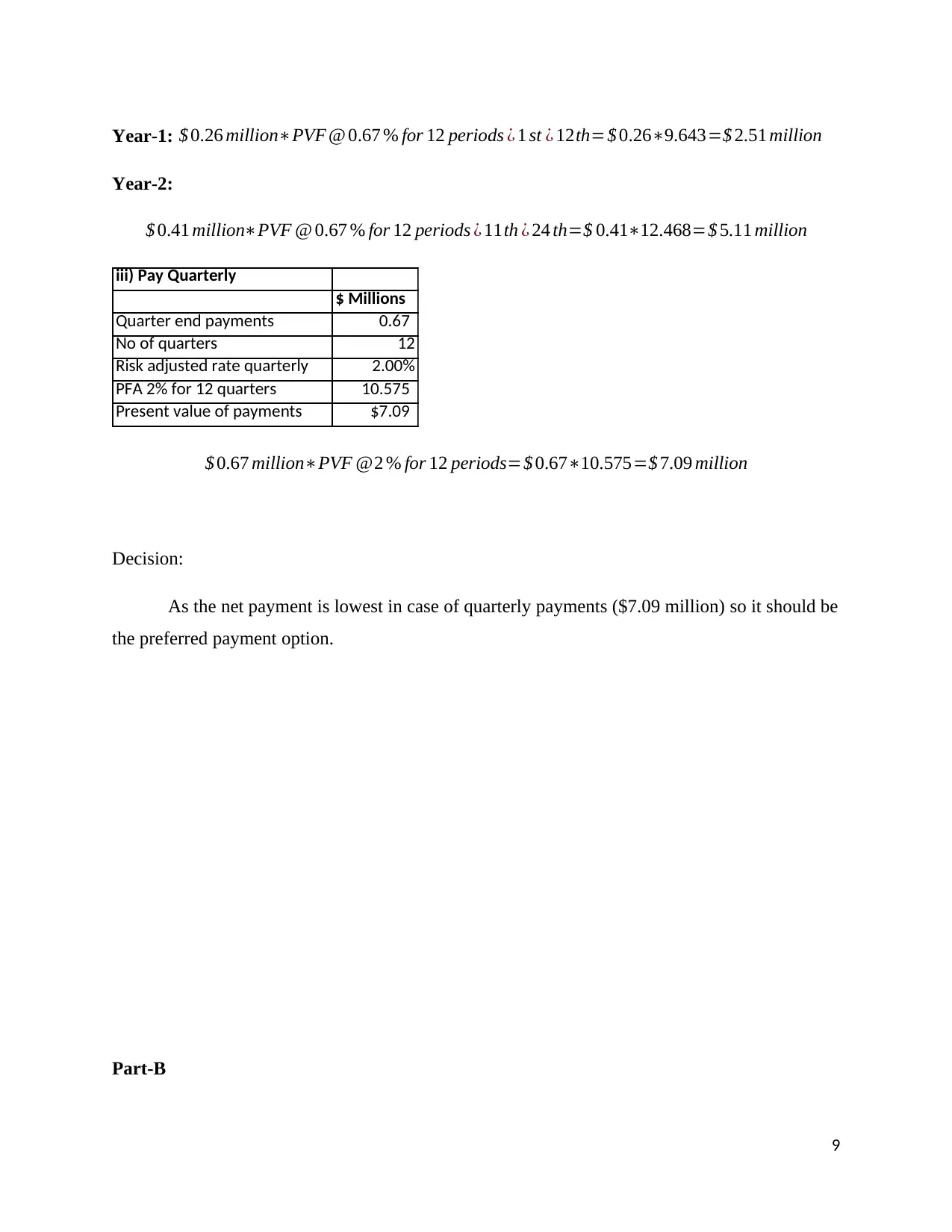
Year-1: $ 0.26 million∗PVF @ 0.67 % for 12 periods ¿ 1 st ¿ 12th=$ 0.26∗9.643=$ 2.51 million
Year-2:
$ 0.41 million∗PVF @ 0.67 % for 12 periods ¿ 11th ¿ 24 th=$ 0.41∗12.468=$ 5.11 million
iii) Pay Quarterly
$ Millions
Quarter end payments 0.67
No of quarters 12
Risk adjusted rate quarterly 2.00%
PFA 2% for 12 quarters 10.575
Present value of payments $7.09
$ 0.67 million∗PVF @2 % for 12 periods=$ 0.67∗10.575=$ 7.09 million
Decision:
As the net payment is lowest in case of quarterly payments ($7.09 million) so it should be
the preferred payment option.
Part-B
9
⊘ This is a preview!⊘
Do you want full access?
Subscribe today to unlock all pages.
Trusted by 1+ million students worldwide
Executive Summary
This report presents an analysis of the capital structure and financial performance of ANZ
Bank. The capital structure of the bank has been static with little or few changes in the
composition of debt and equity. More or less, the debt equity ratio of the bank has been found to
be 0.86:1, which indicates that the bank is using more debt than equity. Further, the return on
equity ratio (11.90%) and EPS (237.1 cents) show improvement in the profitability. The liquidity
position of the bank is also good as shown by the improved liquidity coverage ratio (135%).
Introduction
The report presented here deals with the financial analysis of ANZ Bank. The ANZ Bank
is one of the top most banks operating in Australia and New Zealand. The report presents an
analysis of the capital structure and cost of capital of the bank. Further, the report also puts light
on the financial performance of the bank.
Analysis of the Capital Structure of ANZ
The capital structure of a firm shows the composition of its capital funds. A firm may
arrange funds from various sources which mainly fall in two primary categories such as equity
and debt. Different sources of funds have incurs different costs and have different risk
characteristics. Therefore, it becomes essential for a firm to analyze its capital structure and
optimize the cost of capital and risk.
The capital structure of ANZ Bank for the year 2017 has been analyzed as under:
10
Paraphrase This Document
Need a fresh take? Get an instant paraphrase of this document with our AI Paraphraser
Particulars Amount ($M) % to total
Debt
Deposits and other borrowings 595,611.00
Debt issuances 107,973.00
Total 703,584.00 86%
Equity
Share capital (market cap) 86,352.39
Reserves 37.00
Retained earnings 29,834.00
Total 116,223.39 14%
Grand total 819,807.39
ANZ's current capital structure: 2017
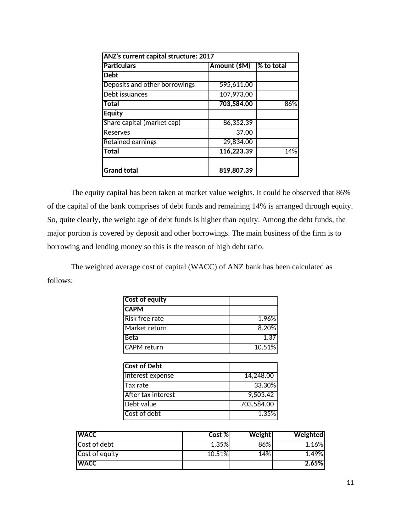
The equity capital has been taken at market value weights. It could be observed that 86%
of the capital of the bank comprises of debt funds and remaining 14% is arranged through equity.
So, quite clearly, the weight age of debt funds is higher than equity. Among the debt funds, the
major portion is covered by deposit and other borrowings. The main business of the firm is to
borrowing and lending money so this is the reason of high debt ratio.
The weighted average cost of capital (WACC) of ANZ bank has been calculated as
follows:
Cost of equity
CAPM
Risk free rate 1.96%
Market return 8.20%
Beta 1.37
CAPM return 10.51%
Cost of Debt
Interest expense 14,248.00
Tax rate 33.30%
After tax interest 9,503.42
Debt value 703,584.00
Cost of debt 1.35%
WACC Cost % Weight Weighted
Cost of debt 1.35% 86% 1.16%
Cost of equity 10.51% 14% 1.49%
WACC 2.65%
11
Debt
Deposits and other borrowings 595,611.00
Debt issuances 107,973.00
Total 703,584.00 86%
Equity
Share capital (market cap) 86,352.39
Reserves 37.00
Retained earnings 29,834.00
Total 116,223.39 14%
Grand total 819,807.39
ANZ's current capital structure: 2017
The equity capital has been taken at market value weights. It could be observed that 86%
of the capital of the bank comprises of debt funds and remaining 14% is arranged through equity.
So, quite clearly, the weight age of debt funds is higher than equity. Among the debt funds, the
major portion is covered by deposit and other borrowings. The main business of the firm is to
borrowing and lending money so this is the reason of high debt ratio.
The weighted average cost of capital (WACC) of ANZ bank has been calculated as
follows:
Cost of equity
CAPM
Risk free rate 1.96%
Market return 8.20%
Beta 1.37
CAPM return 10.51%
Cost of Debt
Interest expense 14,248.00
Tax rate 33.30%
After tax interest 9,503.42
Debt value 703,584.00
Cost of debt 1.35%
WACC Cost % Weight Weighted
Cost of debt 1.35% 86% 1.16%
Cost of equity 10.51% 14% 1.49%
WACC 2.65%
11
The cost of equity has been computed applying the CAPM model. The cost of equity is
10.51% which is higher than the cost of debt of 1.35%. The weight of debt in the total capital of
the bank is 86%. So, the bank is using low cost funds more than the equity which incurs high
cost. Due to this composition, the weighted average cost of capital of the bank is 2.65% which
can be said to be quite low.
The CAPM return provides an approximation to the minimum required rate of return for
the equity investors. The equity investors can analyze that whether the firm is able to provide
them adequate return by comparing the CAPM return with the actual return on equity (ROE) of
the firm (Hou & Van Dijk, 2018). In the case of ANZ Bank, the CAPM return is 10.51% while
the return on equity is 11.90% (ANZ Bank, 2017), which indicates that the bank has been able to
provide adequate return to its equity investors.
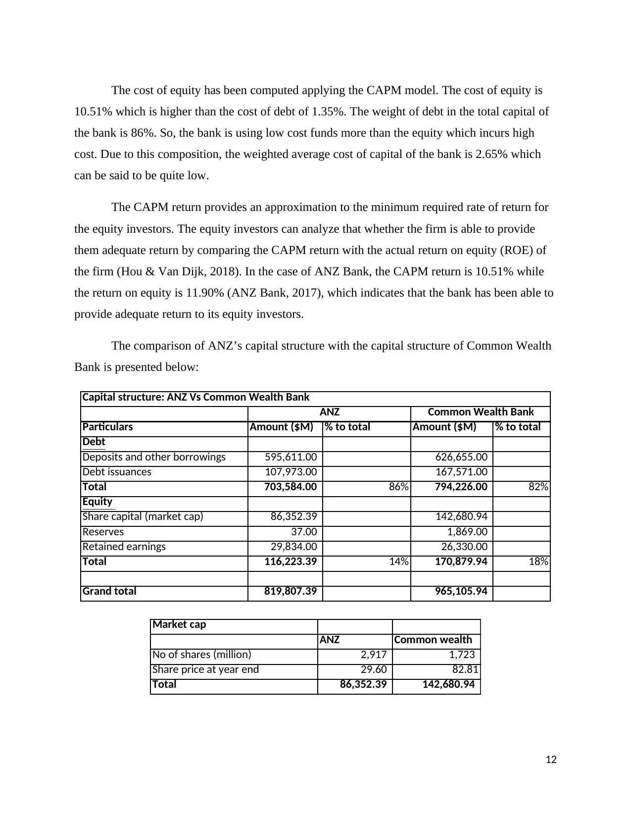
The comparison of ANZ’s capital structure with the capital structure of Common Wealth
Bank is presented below:
Particulars Amount ($M) % to total Amount ($M) % to total
Debt
Deposits and other borrowings 595,611.00 626,655.00
Debt issuances 107,973.00 167,571.00
Total 703,584.00 86% 794,226.00 82%
Equity
Share capital (market cap) 86,352.39 142,680.94
Reserves 37.00 1,869.00
Retained earnings 29,834.00 26,330.00
Total 116,223.39 14% 170,879.94 18%
Grand total 819,807.39 965,105.94
Capital structure: ANZ Vs Common Wealth Bank
ANZ Common Wealth Bank
Market cap
ANZ Common wealth
No of shares (million) 2,917 1,723
Share price at year end 29.60 82.81
Total 86,352.39 142,680.94
12
10.51% which is higher than the cost of debt of 1.35%. The weight of debt in the total capital of
the bank is 86%. So, the bank is using low cost funds more than the equity which incurs high
cost. Due to this composition, the weighted average cost of capital of the bank is 2.65% which
can be said to be quite low.
The CAPM return provides an approximation to the minimum required rate of return for
the equity investors. The equity investors can analyze that whether the firm is able to provide
them adequate return by comparing the CAPM return with the actual return on equity (ROE) of
the firm (Hou & Van Dijk, 2018). In the case of ANZ Bank, the CAPM return is 10.51% while
the return on equity is 11.90% (ANZ Bank, 2017), which indicates that the bank has been able to
provide adequate return to its equity investors.
The comparison of ANZ’s capital structure with the capital structure of Common Wealth
Bank is presented below:
Particulars Amount ($M) % to total Amount ($M) % to total
Debt
Deposits and other borrowings 595,611.00 626,655.00
Debt issuances 107,973.00 167,571.00
Total 703,584.00 86% 794,226.00 82%
Equity
Share capital (market cap) 86,352.39 142,680.94
Reserves 37.00 1,869.00
Retained earnings 29,834.00 26,330.00
Total 116,223.39 14% 170,879.94 18%
Grand total 819,807.39 965,105.94
Capital structure: ANZ Vs Common Wealth Bank
ANZ Common Wealth Bank
Market cap
ANZ Common wealth
No of shares (million) 2,917 1,723
Share price at year end 29.60 82.81
Total 86,352.39 142,680.94
12
⊘ This is a preview!⊘
Do you want full access?
Subscribe today to unlock all pages.
Trusted by 1+ million students worldwide
1 out of 18


Your All-in-One AI-Powered Toolkit for Academic Success.
+13062052269
info@desklib.com
Available 24*7 on WhatsApp / Email
![[object Object]](/_next/static/media/star-bottom.7253800d.svg)
Unlock your academic potential
Copyright © 2020–2026 A2Z Services. All Rights Reserved. Developed and managed by ZUCOL.