University Assignment: Decision Analysis, CVP and Regression Analysis

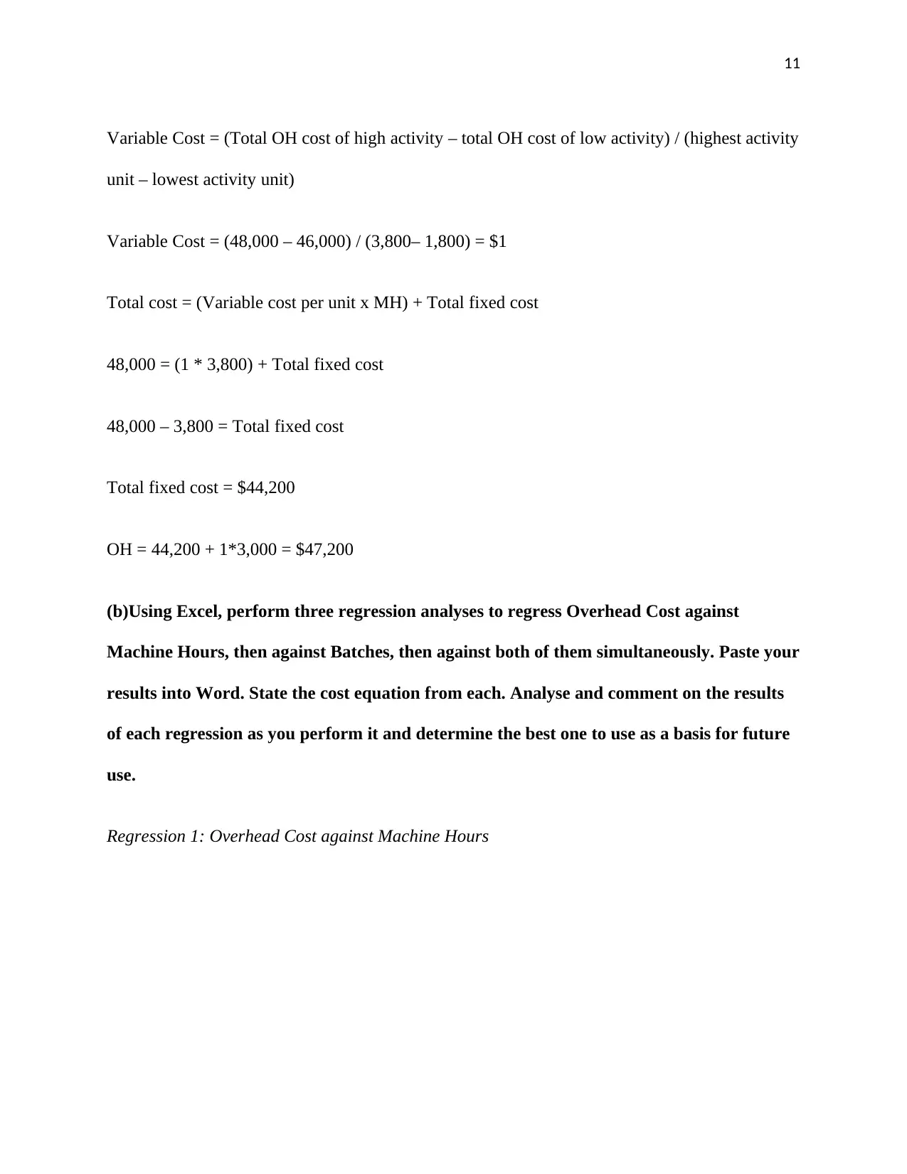
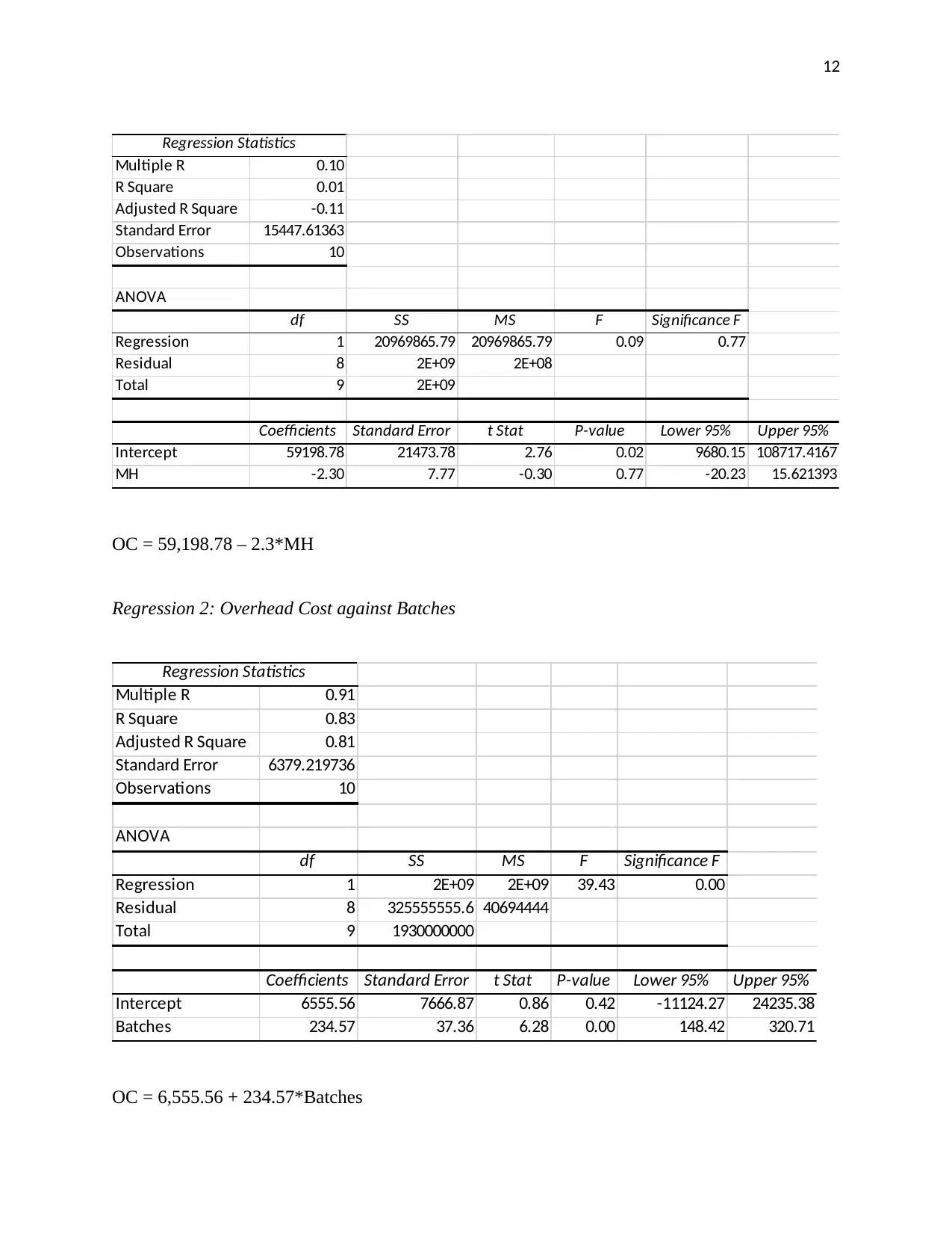
This assignment solution covers key concepts in business development, including decision analysis, value of information, and Monte Carlo simulation. It begins with a discussion of utility functions and standard gambles, followed by a decision matrix analysis of investment strategies. The solution then explores the value of information, calculating posterior probabilities and expected net gains. A Monte Carlo simulation is used to determine expected average monthly profit. Furthermore, the assignment delves into regression analysis, estimating overhead costs using the high-low method and performing regression analyses to determine the best cost equation. Finally, it concludes with a CVP analysis, calculating contribution margins, break-even points, and profit calculations under different scenarios. The solution provides detailed calculations and explanations for each question, offering a comprehensive guide for students studying business development and related topics.

1
Subject code:
Subject name:
Student’s name:
Student number:
Assessment item number:

2
Assignment 3
QUESTION 1 Decision Analysis
(a) Discuss how a utility function can be assessed. What is a standard gamble and how is it
used in determining utility values?
Utility functions are assessed by:
a. Identifying the worst and best attribute levels
b. Assigning utility of zero to worst outcome and 1 to best outcome
c. Naming the desirable outcome at 50:50
The Standard Gamble (SG) measures the preference of an individual under uncertainty. It is used
to express the outcome of different choices in utility values. Standard gamble determines the
mean probability when a respondent is indifferent between accepting a gamble and continuing
with the current situation.
(b) Alan Barnes invests primarily in the share market. Recently he has become concerned
about the share market as a good investment. During the next year he must decide whether
to invest $10,000 in the share market or in a government bond at an interest rate of 9%.
Alan expects the share market to be good, fair or bad, giving a return of 14%, 8% or 0%
respectively on his money.

3
1. Develop a decision matrix showing the two possible strategies, the three states of the
share market and the monetary gains or losses under the six possible action-state scenarios.
Table 1: Data
Profit Shares Bonds
Probability 50% 50%
Good 14% 9%
Fair 8% 9%
Poor 0% 9%
Table 2: Results
EMV Minimum Maximum
0.115 0.09 0.14
0.085 0.08 0.09
0.045 0 0.09
Maximum 0.115 0.09 0.14
Table 3: Criterion of regret
Regret
Shares Bonds Expected Maximum
Probability 0.5 0.5

4
Good 0% 0 0 0
Fair 0.06 0 0.03 0.06
Poor 0.14 0 0.07 0.14
Minimum 0 0
2. Which alternative would an optimist choose? The share market
3. Which alternative would a pessimist choose? The bonds market
4. Which alternative is indicated by the criterion of regret? There is no alternative
indicated under the criterion of regret.
5. Assuming probability of a good market = 0.4, a fair market = 0.4 and a bad market = 0.2,
using expected monetary values what is the optimum action?
Data Results
Profit Shares Bonds EMV Minimum Maximum
Probability 50% 50%
Good 40% 9% 0.245 0.09 0.4
Fair 40% 9% 0.245 0.09 0.4
Poor 20% 9% 0.145 0.09 0.2
Maximum 0.245 0.09 0.4
The optimum action would be to invest wholly in the share market.
6. What is the expected value of perfect information?

5
Data
Profit Shares Bonds
Probability 50% 50%
Good 40% 9%
Fair 40% 9%
Poor 20% 9%
Expected Value of Perfect Information
Column
best 40% 9%
Expected value with prefer information = (50%*40%) + (50%+9%) = 0.245
QUESTION 2 Value of information
(a) What should Jerry do?
Jerry should produce the new type of electric razor. The expected returns would be $20,000. The
justification is as seen below:

6
0.5
Favourable 4 100000
20000 100000
Invest 2
0 0.5
20000 Unfavourable 5 -60000
1 -60000
2
Do nothing 3 0
0
(b)Revise the prior probabilities in light of his friend’s track record.
0.5
Favourable 5 100000
20000 100000
Invest 2
0.5
Unfavourable 6 -60000
-60000
Don’t invest 3 0
20000
1
2 0.7
Favourable 9 100000
0.5 52000 100000
Correct 7
0 0.3
Unfavourable 10 -60000
12000 -60000
Friend 4
0.2
Favourable 11 100000
0.5 -28000 100000
Incorrect 8
0 0.8
Unfavourable 12 -60000
-60000
(c)What is the posterior probability of a good market given that his friend has provided an
unfavourable market prediction?

7
Posterior probability = 1 - 0.3*0.8 = 1 - 0.24 = 0.76
(d)What is the expected net gain or loss from engaging his friend to conduct the market
research? Should his friend be engaged? Why?
The expected net gain from engaging his friends to conduct market research is $12,000. Since
this is lower than if he had not consulted, then he should not consult his friend.
QUESTION 3 Monte Carlo Simulation
(a)Using Excel set up a model to simulate the next 12 months to determine the expected
average monthly profit for the year. You need to have loaded the Analysis Toolpak Add-In
to your version of Excel. You must keep the data separate from the model. The model
should show only formulas, no numbers whatsoever except for the month number.

8
Table 1: Results
16
17
18
19
20
21
22
23
24
25
26
27
28
29
30
31
A B C D E F G H
MODEL
Selling Profit Fixed
Month RN1 Demand Price RN2 Margin Costs Profit
1 0.46 200 160 0.04 0.2 2000 4,521.25$
2 0.15 120 175 0.52 0.3 2000 3,284.49$
3 0.49 200 180 0.06 0.2 2000 5,399.45$
4 0.65 200 168 0.96 0.3 2000 7,949.70$
5 0.58 200 173 0.14 0.2 2000 5,397.25$
6 0.31 200 168 0.88 0.3 2000 7,680.33$
7 0.10 120 173 0.64 0.3 2000 3,480.95$
8 0.16 120 160 0.31 0.2 2000 2,443.32$
9 0.94 200 160 0.72 0.3 2000 6,719.92$
10 0.41 200 178 0.31 0.2 2000 6,237.04$
11 0.53 200 179 0.42 0.2 2000 6,649.84$
12 0.92 200 173 0.42 0.2 2000 6,375.70$
Profit average 5,511.60$
Table 2: Formulae
16
17
18
19
20
21
22
23
24
25
26
27
28
29
30
31
A B C D E F G H
MODEL
Selling Profit Fixed
Month RN1 Demand Price RN2 Margin Costs Profit
1 =RAND() =LOOKUP(B19,$A$5:$A$10,$C$5:$C$10)=RANDBETWEEN($G$4,$H$4) =RAND() =0.2+(0.3-0.2)*E19 =$G$5 =C19*D19*F19-G19
2 =RAND() =LOOKUP(B20,$A$5:$A$10,$C$5:$C$10)=RANDBETWEEN($G$4,$H$4) =RAND() =0.2+(0.3-0.2)*E20 =$G$5 =C20*D20*F20-G20
3 =RAND() =LOOKUP(B21,$A$5:$A$10,$C$5:$C$10)=RANDBETWEEN($G$4,$H$4) =RAND() =0.2+(0.3-0.2)*E21 =$G$5 =C21*D21*F21-G21
4 =RAND() =LOOKUP(B22,$A$5:$A$10,$C$5:$C$10)=RANDBETWEEN($G$4,$H$4) =RAND() =0.2+(0.3-0.2)*E22 =$G$5 =C22*D22*F22-G22
5 =RAND() =LOOKUP(B23,$A$5:$A$10,$C$5:$C$10)=RANDBETWEEN($G$4,$H$4) =RAND() =0.2+(0.3-0.2)*E23 =$G$5 =C23*D23*F23-G23
6 =RAND() =LOOKUP(B24,$A$5:$A$10,$C$5:$C$10)=RANDBETWEEN($G$4,$H$4) =RAND() =0.2+(0.3-0.2)*E24 =$G$5 =C24*D24*F24-G24
7 =RAND() =LOOKUP(B25,$A$5:$A$10,$C$5:$C$10)=RANDBETWEEN($G$4,$H$4) =RAND() =0.2+(0.3-0.2)*E25 =$G$5 =C25*D25*F25-G25
8 =RAND() =LOOKUP(B26,$A$5:$A$10,$C$5:$C$10)=RANDBETWEEN($G$4,$H$4) =RAND() =0.2+(0.3-0.2)*E26 =$G$5 =C26*D26*F26-G26
9 =RAND() =LOOKUP(B27,$A$5:$A$10,$C$5:$C$10)=RANDBETWEEN($G$4,$H$4) =RAND() =0.2+(0.3-0.2)*E27 =$G$5 =C27*D27*F27-G27
10 =RAND() =LOOKUP(B28,$A$5:$A$10,$C$5:$C$10)=RANDBETWEEN($G$4,$H$4) =RAND() =0.2+(0.3-0.2)*E28 =$G$5 =C28*D28*F28-G28
11 =RAND() =LOOKUP(B29,$A$5:$A$10,$C$5:$C$10)=RANDBETWEEN($G$4,$H$4) =RAND() =0.2+(0.3-0.2)*E29 =$G$5 =C29*D29*F29-G29
12 =RAND() =LOOKUP(B30,$A$5:$A$10,$C$5:$C$10)=RANDBETWEEN($G$4,$H$4) =RAND() =0.2+(0.3-0.2)*E30 =$G$5 =C30*D30*F30-G30
Profit average =AVERAGE(H19:H30)

9
(b)Provide the average monthly profit to Ajax Tyres over the 12-month period.
The average monthly profit as seen in table 1 is $5,511.60
(c)You present your findings to the manager of Ajax Tyres. He thinks that with market
forces he can increase the average selling price by $40 (ie from $200 to $220) without losing
sales. However he does suggest that the profit margin would then increase from 22% to
32%.
16
17
18
19
20
21
22
23
24
25
26
27
28
29
30
31
A B C D E F G H
MODEL
Selling Profit Fixed
Month RN1 Demand Price RN2 Margin Costs Profit
1 0.899464096 200 214 0.458825 0.2 2000 8,523.77$
2 0.150309382 120 213 0.782066 0.3 2000 5,110.96$
3 0.939565333 200 206 0.926011 0.3 2000 10,055.17$
4 0.6304883 200 209 0.784928 0.3 2000 9,641.00$
5 0.262048794 200 207 0.529999 0.3 2000 8,474.19$
6 0.272227262 200 203 0.967227 0.3 2000 10,046.94$
7 0.513738928 200 200 0.027442 0.2 2000 6,109.77$
8 0.860827248 200 218 0.151551 0.2 2000 7,380.76$
9 0.56451984 200 214 0.237897 0.2 2000 7,578.20$
10 0.617149483 200 214 0.45493 0.2 2000 8,507.10$
11 0.331056192 200 201 0.724339 0.3 2000 8,951.84$
12 0.374034171 200 220 0.324356 0.2 2000 8,227.17$
Profit average 8,217.24$
INTERNAL MEMO
To: Manager, Sales
From: John Doe, Snr. Sales Officer

10
Subject: Change in sales review
Date: 19th September 2018
It is of my belief that the new prices suggested will bring a positive impact to the average
monthly prices. The increase in selling price by $40 will see the company increase its profit
margin from 22% to 32%.
Simulating the new selling price and the new profit margins, using the same model it will be seen
that there was an increase in the average monthly profits from $5,511 to $8,217. Therefore, I
wholly support the new move to increase the selling price from $160 - $180 to $200 - $220.
Thank you for your time,
John Connor,
Snr. Sales Officer.
QUESTION 4 Regression Analysis
(a)Using the high-low method to estimate support overhead costs based on machine hours
(MH), what would be the estimated support overhead costs (to the nearest $) for a month in
which 3,000 machine hours were used?

11
Variable Cost = (Total OH cost of high activity – total OH cost of low activity) / (highest activity
unit – lowest activity unit)
Variable Cost = (48,000 – 46,000) / (3,800– 1,800) = $1
Total cost = (Variable cost per unit x MH) + Total fixed cost
48,000 = (1 * 3,800) + Total fixed cost
48,000 – 3,800 = Total fixed cost
Total fixed cost = $44,200
OH = 44,200 + 1*3,000 = $47,200
(b)Using Excel, perform three regression analyses to regress Overhead Cost against
Machine Hours, then against Batches, then against both of them simultaneously. Paste your
results into Word. State the cost equation from each. Analyse and comment on the results
of each regression as you perform it and determine the best one to use as a basis for future
use.
Regression 1: Overhead Cost against Machine Hours

12
Regression Statistics
Multiple R 0.10
R Square 0.01
Adjusted R Square -0.11
Standard Error 15447.61363
Observations 10
ANOVA
df SS MS F Significance F
Regression 1 20969865.79 20969865.79 0.09 0.77
Residual 8 2E+09 2E+08
Total 9 2E+09
Coefficients Standard Error t Stat P-value Lower 95% Upper 95%
Intercept 59198.78 21473.78 2.76 0.02 9680.15 108717.4167
MH -2.30 7.77 -0.30 0.77 -20.23 15.621393
OC = 59,198.78 – 2.3*MH
Regression 2: Overhead Cost against Batches
Regression Statistics
Multiple R 0.91
R Square 0.83
Adjusted R Square 0.81
Standard Error 6379.219736
Observations 10
ANOVA
df SS MS F Significance F
Regression 1 2E+09 2E+09 39.43 0.00
Residual 8 325555555.6 40694444
Total 9 1930000000
Coefficients Standard Error t Stat P-value Lower 95% Upper 95%
Intercept 6555.56 7666.87 0.86 0.42 -11124.27 24235.38
Batches 234.57 37.36 6.28 0.00 148.42 320.71
OC = 6,555.56 + 234.57*Batches