Decision Analysis, Value of Information, and Cost Analysis Homework

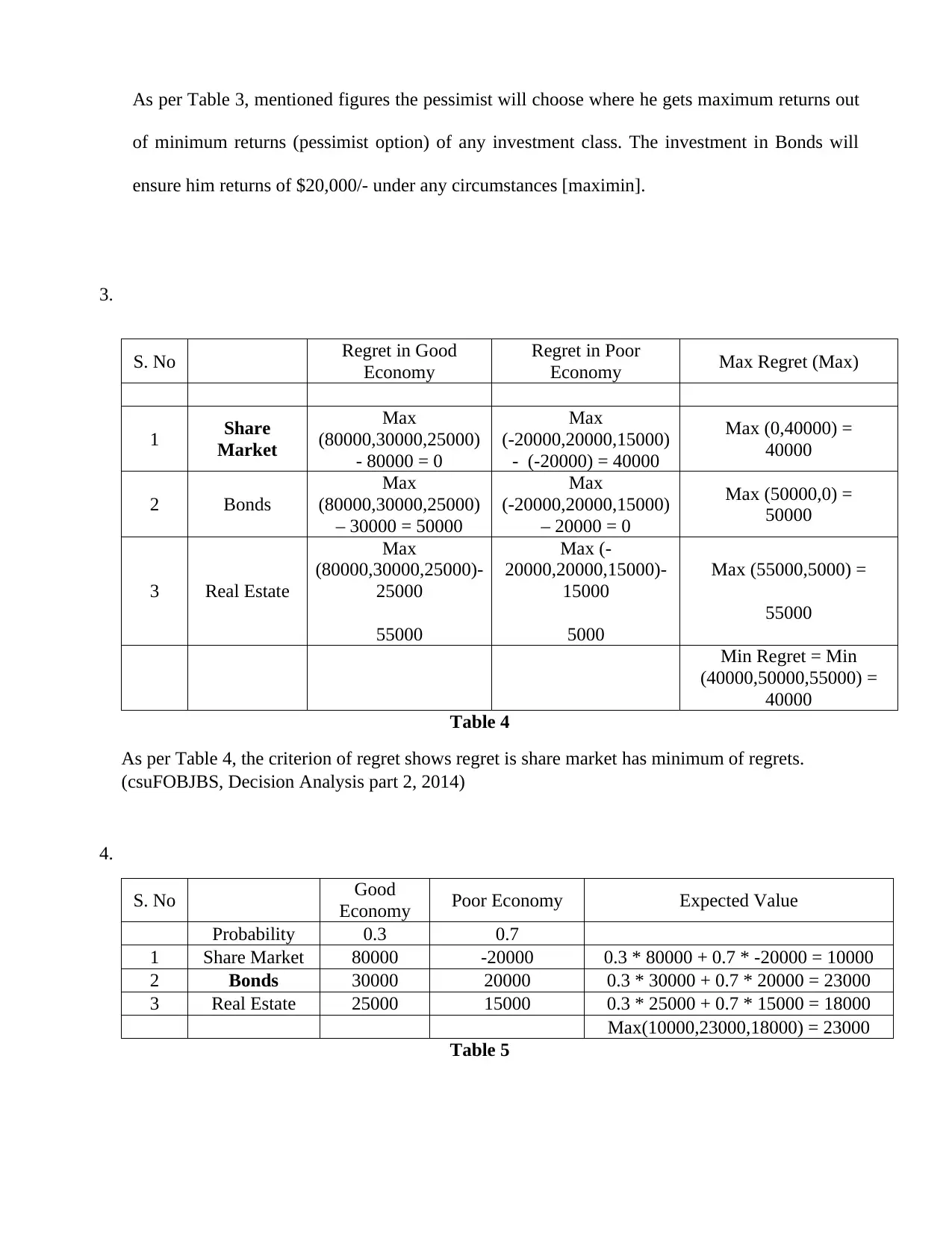
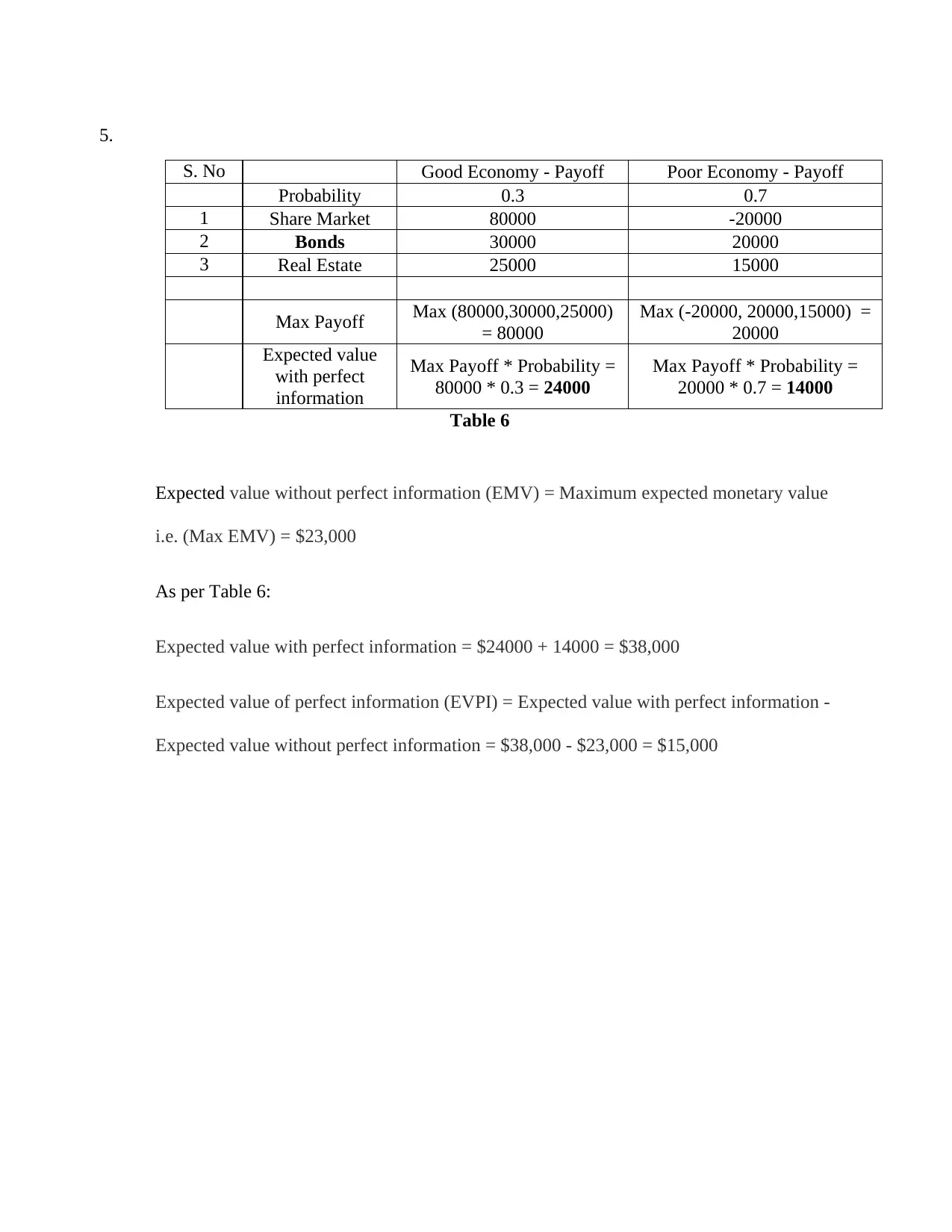
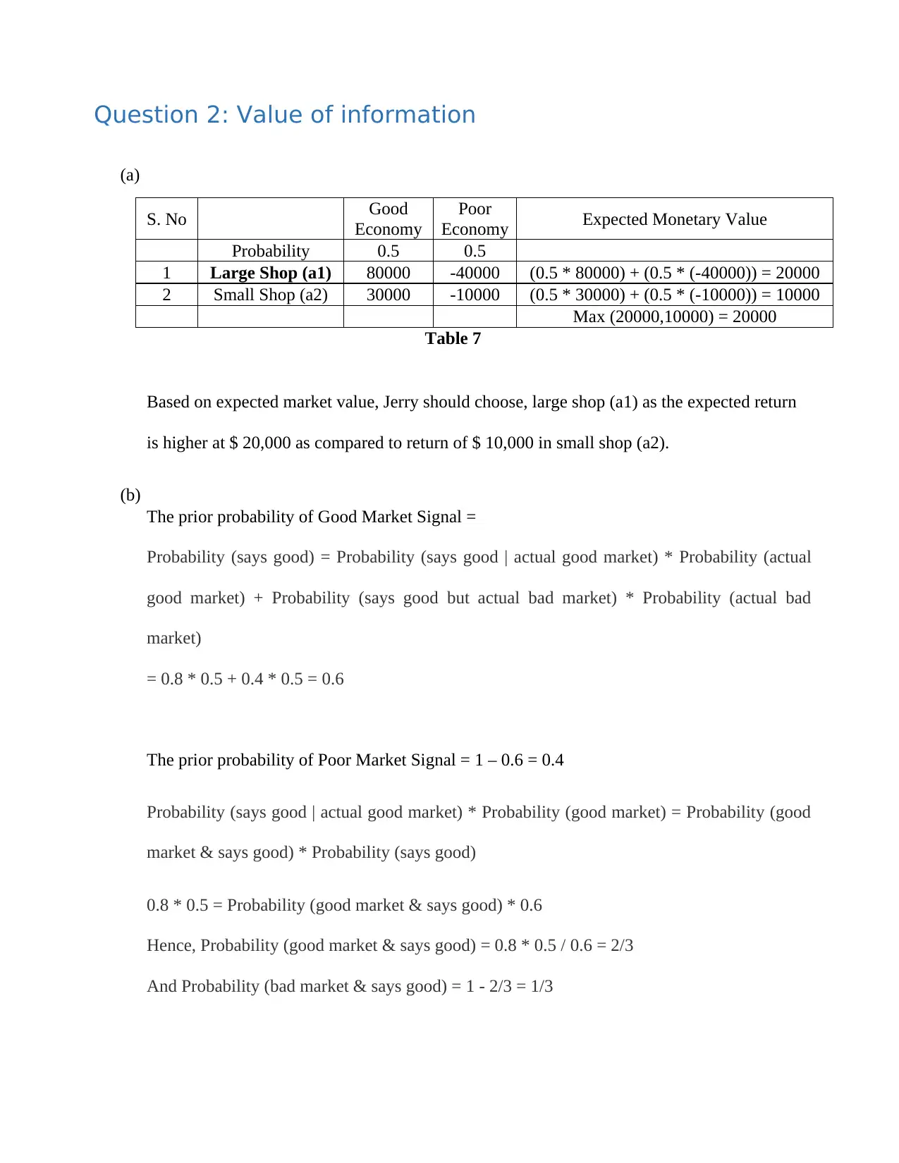
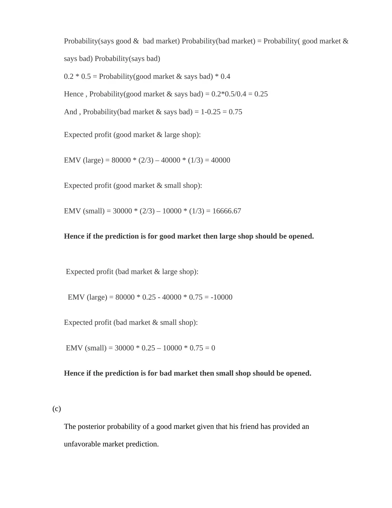
This assignment solution covers various aspects of decision analysis, starting with decision-making under certainty, risk, and uncertainty, and exploring methods like maximax, maximin, and regret analysis. It then delves into the value of information, providing calculations for prior and posterior probabilities to determine the optimal decision based on market signals. The solution also includes a Monte Carlo simulation to assess potential profits under different scenarios and regression analysis to determine cost behavior. Finally, the assignment addresses cost-volume-profit (CVP) analysis to understand the relationship between costs, volume, and profit. The solution uses tables and calculations to illustrate the concepts and provides a comprehensive overview of the decision-making process in a business context.

Student ID:
Student Name:
Course ID:
Instructor Name:

Table of Contents
Question 1: Decision Analysis.............................................................................................................................3
Question 2: Value of information........................................................................................................................7
Question 3: Monte Carlo Simulation...................................................................................................................9
Question 4: Regression Analysis........................................................................................................................10
Question 5: CVP Analysis...................................................................................................................................14
References........................................................................................................................................................17

Question 1: Decision Analysis
(a)
Decision Making under Certainty
The decision making under certainty is identifying the best option or alternative and to optimize the
outcome. In decision making under certainty the various outcomes are known and their
values are certain. Hence the task is merely to optimize the required criterion such as to minimize the
cost or to maximize the profits. Since perfect information is rarely available on all the various
parameters impacting decision, hence this technique (decision making under certainty) is less often
used. Moreover in normal circumstances there is cost of information hence this cost aspect also needs
to be analyzed and expected value of perfect information (EVPI) needs to be calculated. E.g. If you
want to make a decision of buying a soap ‘Dove’ or ‘Pears’ and the benefits of both the soaps are
same, then cost of soaps are considered. Pears soap is cheaper than Dove, so the decision will be to
buy Pears.
Decision Making under Risk
In decision making under risk, the outcomes are known as also the probabilities of occurrence are
known and in such scenario, instead of optimizing the outcome we instead optimize the expected
monetary value (EMV) of outcome. The highest EMV will be selected. E.g. if there is 1% probability
of earning $1000 in option A while there is 90% probability of earning $ 50 in option B , the option
B shall be preferred as the EMV of option B is $ 45 (90% of $ 45) rather than EMV of $ 10 in option
A (1% of $ 1000).
Decision Making under Complete Uncertainty

Under uncertainty, only the outcomes are known but not their probability. Here the selection is based
on maximax, maximin or equally likely methods for the positive or cautious or neutral perspective/s
respectively.
(b)
Good Economy Poor Economy
Probability 0.3 0.7
Share Market 80000 -20000
Bonds 30000 20000
Real Estate 25000 15000
Table 1
1.
S. No Good Economy Poor Economy Best Result (Max)
1 Share
Market 80000 -20000 80000 (Max 80000,-20000)
2 Bonds 30000 20000 30000 (Max 30000,20000)
3 Real Estate 25000 15000 25000 (Max 25000,15000)
80000
(Max(80000,30000,25000))
Table 2
As per Table 2, the optimist would choose share market investment because the share market
returns (under best conditions) are the maximum of the maximum returns in any investment
group i.e. return of $80,000 [maximax] (csuFOBJBS, Decision Analysis part 1, 2014)
2.
S. No Good Economy Poor Economy Best Result (Min)
1 Share Market 80000 -20000 -20000 (Min 80000,-20000)
2 Bonds 30000 20000 20000 (Min 30000,20000)
3 Real Estate 25000 15000 15000 (Min 25000,15000)
20000
(Max(-20000,20000,15000))
Table 3

As per Table 3, mentioned figures the pessimist will choose where he gets maximum returns out
of minimum returns (pessimist option) of any investment class. The investment in Bonds will
ensure him returns of $20,000/- under any circumstances [maximin].
3.
S. No Regret in Good
Economy
Regret in Poor
Economy Max Regret (Max)
1 Share
Market
Max
(80000,30000,25000)
- 80000 = 0
Max
(-20000,20000,15000)
- (-20000) = 40000
Max (0,40000) =
40000
2 Bonds
Max
(80000,30000,25000)
– 30000 = 50000
Max
(-20000,20000,15000)
– 20000 = 0
Max (50000,0) =
50000
3 Real Estate
Max
(80000,30000,25000)-
25000
55000
Max (-
20000,20000,15000)-
15000
5000
Max (55000,5000) =
55000
Min Regret = Min
(40000,50000,55000) =
40000
Table 4
As per Table 4, the criterion of regret shows regret is share market has minimum of regrets.
(csuFOBJBS, Decision Analysis part 2, 2014)
4.
S. No Good
Economy Poor Economy Expected Value
Probability 0.3 0.7
1 Share Market 80000 -20000 0.3 * 80000 + 0.7 * -20000 = 10000
2 Bonds 30000 20000 0.3 * 30000 + 0.7 * 20000 = 23000
3 Real Estate 25000 15000 0.3 * 25000 + 0.7 * 15000 = 18000
Max(10000,23000,18000) = 23000
Table 5

As per Table 5, based on probability of a good economy = 0.3, the expected monetary values
suggest optimum action of investing in Bonds with expected return of $23,000

5.
S. No Good Economy - Payoff Poor Economy - Payoff
Probability 0.3 0.7
1 Share Market 80000 -20000
2 Bonds 30000 20000
3 Real Estate 25000 15000
Max Payoff Max (80000,30000,25000)
= 80000
Max (-20000, 20000,15000) =
20000
Expected value
with perfect
information
Max Payoff * Probability =
80000 * 0.3 = 24000
Max Payoff * Probability =
20000 * 0.7 = 14000
Table 6
Expected value without perfect information (EMV) = Maximum expected monetary value
i.e. (Max EMV) = $23,000
As per Table 6:
Expected value with perfect information = $24000 + 14000 = $38,000
Expected value of perfect information (EVPI) = Expected value with perfect information -
Expected value without perfect information = $38,000 - $23,000 = $15,000

Question 2: Value of information
(a)
S. No Good
Economy
Poor
Economy Expected Monetary Value
Probability 0.5 0.5
1 Large Shop (a1) 80000 -40000 (0.5 * 80000) + (0.5 * (-40000)) = 20000
2 Small Shop (a2) 30000 -10000 (0.5 * 30000) + (0.5 * (-10000)) = 10000
Max (20000,10000) = 20000
Table 7
Based on expected market value, Jerry should choose, large shop (a1) as the expected return
is higher at $ 20,000 as compared to return of $ 10,000 in small shop (a2).
(b)
The prior probability of Good Market Signal =
Probability (says good) = Probability (says good | actual good market) * Probability (actual
good market) + Probability (says good but actual bad market) * Probability (actual bad
market)
= 0.8 * 0.5 + 0.4 * 0.5 = 0.6
The prior probability of Poor Market Signal = 1 – 0.6 = 0.4
Probability (says good | actual good market) * Probability (good market) = Probability (good
market & says good) * Probability (says good)
0.8 * 0.5 = Probability (good market & says good) * 0.6
Hence, Probability (good market & says good) = 0.8 * 0.5 / 0.6 = 2/3
And Probability (bad market & says good) = 1 - 2/3 = 1/3

Probability(says good & bad market) Probability(bad market) = Probability( good market &
says bad) Probability(says bad)
0.2 * 0.5 = Probability(good market & says bad) * 0.4
Hence , Probability(good market & says bad) = 0.2*0.5/0.4 = 0.25
And , Probability(bad market & says bad) = 1-0.25 = 0.75
Expected profit (good market & large shop):
EMV (large) = 80000 * (2/3) – 40000 * (1/3) = 40000
Expected profit (good market & small shop):
EMV (small) = 30000 * (2/3) – 10000 * (1/3) = 16666.67
Hence if the prediction is for good market then large shop should be opened.
Expected profit (bad market & large shop):
EMV (large) = 80000 * 0.25 - 40000 * 0.75 = -10000
Expected profit (bad market & small shop):
EMV (small) = 30000 * 0.25 – 10000 * 0.75 = 0
Hence if the prediction is for bad market then small shop should be opened.
(c)
The posterior probability of a good market given that his friend has provided an
unfavorable market prediction.

Probability(says good & bad market) Probability(bad market) = Probability(good market &
says bad ) Probability(says bad)
0.2 * 0.5=Probability ( good market & says bad ) * 0.4
Hence, Probability(good market & says bad ) = 0.2 * 0.5 / 0.4 = 0.25
Hence, Probability( bad market & says bad ) = 1 - 0.25 = 0.75
Therefore 0.25 is the required probability
(d)
After engaging his friend the expected monetary value, i.e. EMV (info) improves to $ 24000
from $ 20000 previously. Hence he stands to gain $ 4000. However, there is cost of
information i.e. $ 3000 so his net gain would be $ 1000 if he engages his friend’s services.
(csuFOBJBS, Value of information v2, 2015)
Question 3: Monte Carlo Simulation
Data
Selling Price: $ 60 to $ 80 (uniform distribution)
Fixed Cost $ 1500 / month
Profit Margin: 20% to 30% of selling price
Prob Cum Probability Demand
0.05 0.05 100
0.10 0.15 120
0.20 0.35 140
0.30 0.65 160
0.25 0.9 180
0.10 1 200
Table 8

Monthly Demand: LOOKUP(RAND(), Cumm Probability, Demand)
Profit Margin: 20% (Minimum profit) + 30%-20% (Max margin – Min Margin) * Rand()
Selling price = =RANDBETWEEN (Min Selling price, Maximum Selling price)
Monthly Profit = Monthly Demand * Profit Margin * Selling price – Fixed Cost
Month Monthly Demand Profit Margin Selling Price Monthly Profit
1 100 0.266360392 70 364.52
2 140 0.247115827 65 2248.45
3 100 0.215591232 65 1401.34
4 140 0.230139687 78 2513.13
5 140 0.233413401 63 2058.71
6 160 0.255822859 62 2537.76
7 140 0.296303417 65 2696.36
8 120 0.28794513 64 2211.42
9 120 0.244070117 71 2079.48
10 120 0.243390276 70 2044.48
11 120 0.260346493 73 2280.64
12 160 0.240350633 61 2345.82
Table 9
Question 4: Regression Analysis
Month OH Cost MH Batches
1 $80,000 2,200 300
2 40,000 2,400 120
3 63,000 2,100 250
4 45,000 2,700 160
5 44,000 2,300 200
6 48,000 3,800 170
7 65,000 3,600 260
8 46,000 1,800 160
9 33,000 3,200 150
10 66,000 2,800 210
Total 530,000 26,900 1,980
Table 10

a) Highest MH = 3800 therefore highest OH Cost = 48000
Lowest MH = 1800 therefore lowest OH Cost = 46000
Variable Cost (per unit) = (Highest OH Cost – Lowest OH cost)/ (Highest MH – Lowest MH)
= (48000 – 46000) / (3800 – 1800)
= 2000 / 2000 = $ 1 per unit
Total Fixed Cost = Highest OH Cost – (Highest MH * Variable Cost)
= 48000 – (3800 * 1)
= 48000 – 3800 = $44200
Cost Volume = Fixed Cost + (Variable Cost * Machine Hours)
= 44200 + (1 * 3000) = 44200 + 3000 = $47200
b) Regression Analysis
i. Overhead Cost against Machine Hours
SUMMARY OUTPUT
Regression Statistics
Multiple R 0.104236344
R Square 0.010865215
Adjusted R
Square -0.112776633
Standard Error 15447.61363
Observations 10
ANOVA
df SS MS F
Significance
F
Regression 1 20969865.79 20969865.79 0.087876521 0.774444342

Residual 8 1909030134 238628766.8
Total 9 1930000000
Coefficients Standard Error t Stat P-value Lower 95% Upper 95%
Lower
95.0%
Upper
95.0%
Intercept 59198.7845 21473.78291 2.75679347 0.024797288 9680.152308 108717.4167 9680.152308
108717.416
7
MH -2.304380856 7.773521992
-
0.296439742 0.774444342 -20.23015471 15.621393
-
20.23015471 15.621393
Y = Intercept + Slope * units
OH= 59198.7845 – 2.304380856 * MH
Since the P value (in table above) is high and R (or R square) is low, hence correlation is low and
result is not statistically significant and not a good fit.
ii. Overhead Cost against Batches
SUMMARY OUTPUT
Regression Statistics
Multiple R
0.91176661
8
R Square
0.83131836
5
Adjusted R
Square
0.81023316
1
Standard Error
6379.21973
6
Observations 10
ANOVA
df SS MS F
Significance
F
Regression 1 1604444444 1604444444
39.4266211
6 0.000238105
Residual 8 325555555.6
40694444.4
4
Total 9 1930000000
Coefficients
Standard
Error t Stat P-value Lower 95% Upper 95% Lower 95.0%
Upper
95.0%
Intercept
6555.55555
6 7666.867952
0.85505001
5
0.41739356
6
-
11124.27365
24235.3847
6 -11124.27365
24235.3847
6
Batches
234.567901
2 37.35715567
6.27906212
4
0.00023810
5 148.4221458
320.713656
7 148.4221458
320.713656
7

Y = Intercept + Slope * units
OH= 6555.555556 + 234.5679012 * Batches
Since the P value (in table above) is low and R (or R square) is high, hence correlation is high and
result is statistically significant and good fit.

iii. Overhead Cost against Machine Hours and Batches
SUMMARY OUTPUT
Regression Statistics
Multiple R 0.912733424
R Square 0.833082304
Adjusted R
Square 0.785391534
Standard Error 6783.92168
Observations 10
ANOVA
df SS MS F Significance F
Regression 2 1607848846 803924423.2
17.4684178
6 0.001900021
Residual 7 322151153.5 46021593.36
Total 9 1930000000
Coefficients Standard Error t Stat P-value Lower 95% Upper 95% Lower 95.0%
Upper
95.0%
Intercept 9205.657918 12704.91845 0.724574341
0.49221531
4 -20836.70036 39248.0162 -20836.70036 39248.0162
MH -0.930666774 3.421799934 -0.271981645
0.79348351
1 -9.021937883
7.16060433
6 -9.021937883
7.16060433
6
Batches 233.827453 39.8202902 5.872068031
0.00061664
8 139.6674291 327.987477 139.6674291 327.987477
OH= 9205.657918 - 0.930666774 * MH + 233.827453 * Batches
Since the P value (in table above) is low and R (or R square) is high, hence correlation is high and
result is statistically significant and good fit.
Using both Machine Hours and Batches, the R square is highest and P value is lowest. Hence this
model should be preferred in future.
c) The best model is OH against both MH & Batches. The second best is OH against Batches.
This is because the Rsquare is highest and p value lowest. Hence the correlation is high.
d) Machine Hours = 2000
Batches = 150

Overhead Cost = 9205.657918 - 0.930666774 * MH + 233.827453 * Batches
= 9205.657918 - (0.930666774 * 2000) + (233.827453 * 150)
= 9205.657918 - 1861.333548 + 35074.11795 = $42418.44232
Question 5: CVP Analysis
Product A Product B Total
Sales price per unit (A) $10 $20
Variable cost per unit
(B) $5 $12
Fixed Cost $4,000
Table 11
(a) Unit Contribution Margin
i. Product A : Sales Price per unit – Variable Cost per unit
: 10 – 5 = $5 per unit
ii. Product B : Sales Price per unit – Variable Cost per unit
: 20 – 12 = $8 per unit
(b) If only Product B is being produced then to break even the number of units are:
: Fixed Cost / Unit Contribution
: 4000 / 8 = 500 units
(c) If only product A is produced then:
Break Even Sales Volume = Fixed Cost / Contribution Margin Ratio

Contribution Margin Ratio = Unit Contribution Margin / Sales Price per unit
= 5 / 10 = 0.50
Hence,
Break Even Sales Volume = 4000 / 0.50 = $8000
(d) If Product A and Product B are produced in the ratio of 2:1
i. Profit before Tax is $ 5000
Fixed Cost = $ 4000
Hence, Contribution = Profit before Tax + Fixed Cost
= $5000 + $4000 = $9000
Total contribution is:
(Unit Contribution Margin for Product A*2)+Unit Contribution Margin for Product B
($5 * 2) + $8 = $10 + $8 = $18
Hence the number of units of Product B required to be produced = 9000 / 18
= 500 units
Since Product A and Product B are produced in the ratio 2:1, so Product A is produced
= 500 * 2 = 1000 units
ii. Profit after Tax is $21000
30 cent in the dollar = 1 - 0.30 = 0.70
Profit before Tax = Profit after Tax / 30 cent in Dollar
= 21000 / 0.70 = 30000

Total contribution for 1 unit B and 2 units of A: $18
Total Units of Product B = (Profit + Fixed Cost) / Variable Cost
= (4000 + 30000) / 18 = 34000 / 18 = 1889 units
Since Product A and Product B are produced in the ratio 2:1:
Total Units of Product A = 1889 * 2 = 3778 units

References
csuFOBJBS. (2014, August 26). Decision Analysis part 1. Retrieved from https://www.youtube.com/watch?
v=kGNJhtmaAWM&feature=youtu.be
csuFOBJBS. (2014, August 26). Decision Analysis part 2. Retrieved from https://www.youtube.com/watch?
v=MNWFhxPHx-o&feature=youtu.be
csuFOBJBS. (2015, March 3). Value of information v2. Retrieved from https://www.youtube.com/watch?
v=m58do9gIhOY&feature=youtu.be