Decision Support Tools Project: Analysis of Business Decision-Making
VerifiedAdded on 2021/06/18
|14
|2833
|367
Project
AI Summary
This project delves into the realm of decision support tools, encompassing a comprehensive analysis of various decision-making processes and techniques. The project begins by outlining the fundamental steps involved in decision-making, followed by a discussion of key concepts such as alternatives and states of nature within decision theory. It then presents a case study involving a vendor's fish sales, utilizing different decision-making criteria like optimist's, pessimist's, Laplace's, and regret criteria, as well as probability-based approaches to determine optimal inventory levels. The project further explores the application of Bayesian analysis in a marketing scenario, calculating expected values and posterior probabilities to assess the viability of a product launch. Additionally, it includes a practical exercise involving an overbooking model for a hotel, illustrating the use of optimization to minimize costs. Finally, the project concludes with regression analyses examining the relationship between car price and mileage/age, providing insights into the factors influencing pricing decisions. The project demonstrates a strong understanding of decision-making principles and their practical application in business contexts.
Running head: DECISION SUPPORT TOOLS
DECISION SUPPORT TOOLS
Name of Student
Name of University
Author Note
DECISION SUPPORT TOOLS
Name of Student
Name of University
Author Note
Paraphrase This Document
Need a fresh take? Get an instant paraphrase of this document with our AI Paraphraser
1DECISION SUPPORT TOOLS
Table of Contents
Question 1........................................................................................................................................2
a)..................................................................................................................................................2
b)..................................................................................................................................................2
c)..................................................................................................................................................3
1...............................................................................................................................................3
2...............................................................................................................................................4
3...............................................................................................................................................4
4...............................................................................................................................................5
5...............................................................................................................................................5
6...............................................................................................................................................6
7...............................................................................................................................................6
Question 2........................................................................................................................................7
Question 3........................................................................................................................................8
Question 4......................................................................................................................................11
Question 5......................................................................................................................................13
2DECISION SUPPORT TOOLS
Question 1.
a)
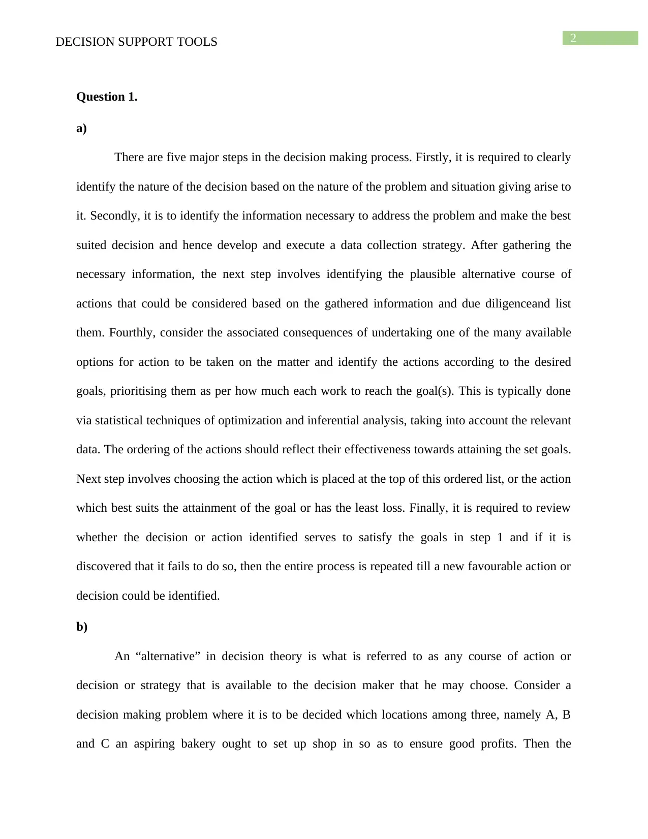
There are five major steps in the decision making process. Firstly, it is required to clearly
identify the nature of the decision based on the nature of the problem and situation giving arise to
it. Secondly, it is to identify the information necessary to address the problem and make the best
suited decision and hence develop and execute a data collection strategy. After gathering the
necessary information, the next step involves identifying the plausible alternative course of
actions that could be considered based on the gathered information and due diligenceand list
them. Fourthly, consider the associated consequences of undertaking one of the many available
options for action to be taken on the matter and identify the actions according to the desired
goals, prioritising them as per how much each work to reach the goal(s). This is typically done
via statistical techniques of optimization and inferential analysis, taking into account the relevant
data. The ordering of the actions should reflect their effectiveness towards attaining the set goals.
Next step involves choosing the action which is placed at the top of this ordered list, or the action
which best suits the attainment of the goal or has the least loss. Finally, it is required to review
whether the decision or action identified serves to satisfy the goals in step 1 and if it is
discovered that it fails to do so, then the entire process is repeated till a new favourable action or
decision could be identified.
b)
An “alternative” in decision theory is what is referred to as any course of action or
decision or strategy that is available to the decision maker that he may choose. Consider a
decision making problem where it is to be decided which locations among three, namely A, B
and C an aspiring bakery ought to set up shop in so as to ensure good profits. Then the
Question 1.
a)
There are five major steps in the decision making process. Firstly, it is required to clearly
identify the nature of the decision based on the nature of the problem and situation giving arise to
it. Secondly, it is to identify the information necessary to address the problem and make the best
suited decision and hence develop and execute a data collection strategy. After gathering the
necessary information, the next step involves identifying the plausible alternative course of
actions that could be considered based on the gathered information and due diligenceand list
them. Fourthly, consider the associated consequences of undertaking one of the many available
options for action to be taken on the matter and identify the actions according to the desired
goals, prioritising them as per how much each work to reach the goal(s). This is typically done
via statistical techniques of optimization and inferential analysis, taking into account the relevant
data. The ordering of the actions should reflect their effectiveness towards attaining the set goals.
Next step involves choosing the action which is placed at the top of this ordered list, or the action
which best suits the attainment of the goal or has the least loss. Finally, it is required to review
whether the decision or action identified serves to satisfy the goals in step 1 and if it is
discovered that it fails to do so, then the entire process is repeated till a new favourable action or
decision could be identified.
b)
An “alternative” in decision theory is what is referred to as any course of action or
decision or strategy that is available to the decision maker that he may choose. Consider a
decision making problem where it is to be decided which locations among three, namely A, B
and C an aspiring bakery ought to set up shop in so as to ensure good profits. Then the
⊘ This is a preview!⊘
Do you want full access?
Subscribe today to unlock all pages.
Trusted by 1+ million students worldwide
3DECISION SUPPORT TOOLS
alternatives available to the decision maker would be either to set up shop at location A or at
location B or at location C out of which best possible course of action is to be determined.
“State of nature” refers to an event or outcome, upon the occurrence of which, the
decision maker has little to no control whatsoever. An example of such an outcome could be
outcomes of random experiments such as getting a “head” as the result of a coin toss or the
chance of blindly drawing an ace of spades from a pack of well shuffled cards.
c)
1.
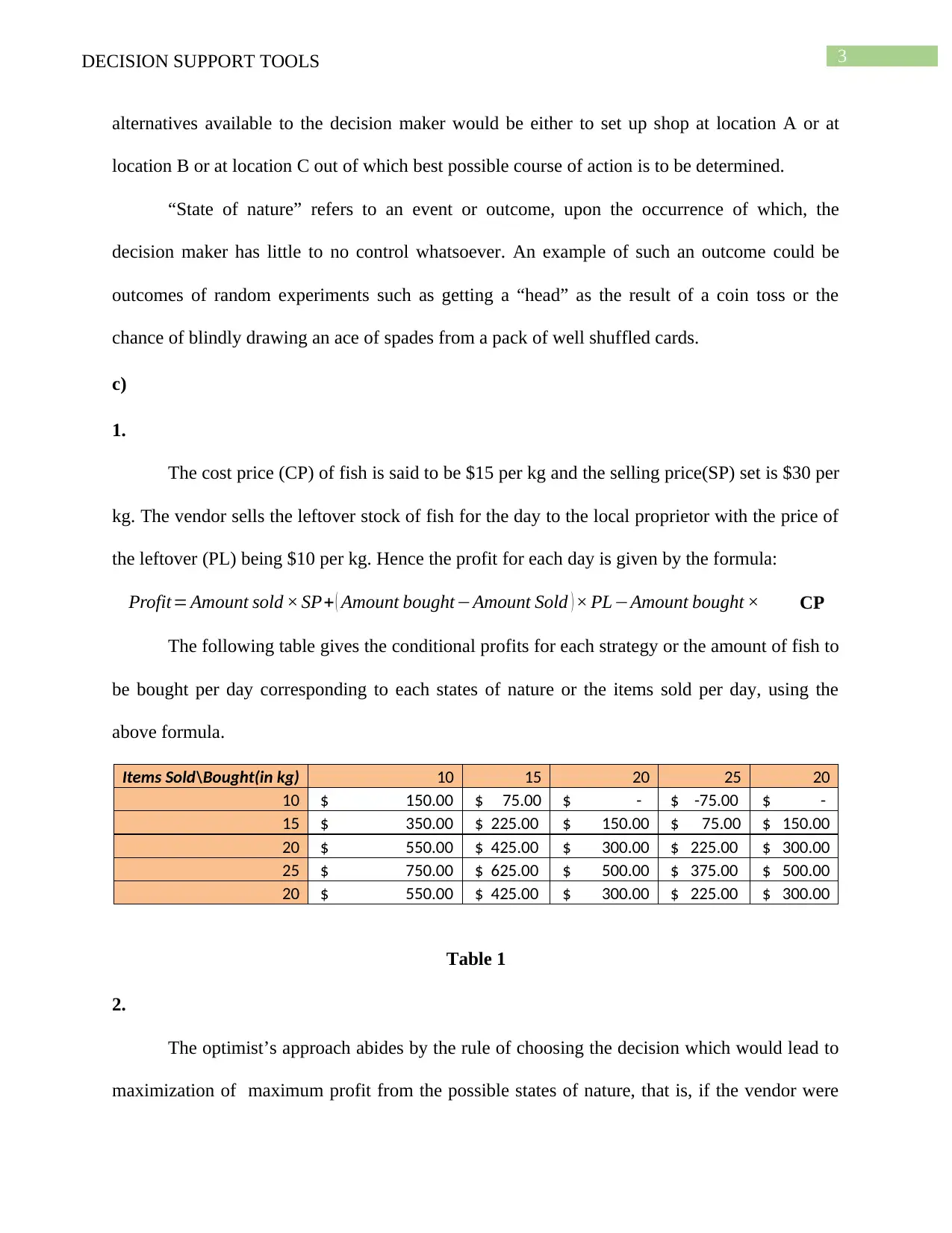
The cost price (CP) of fish is said to be $15 per kg and the selling price(SP) set is $30 per
kg. The vendor sells the leftover stock of fish for the day to the local proprietor with the price of
the leftover (PL) being $10 per kg. Hence the profit for each day is given by the formula:
Profit= Amount sold × SP+ ( Amount bought−Amount Sold ) × PL−Amount bought × CP
The following table gives the conditional profits for each strategy or the amount of fish to
be bought per day corresponding to each states of nature or the items sold per day, using the
above formula.
Items Sold\Bought(in kg) 10 15 20 25 20
10 $ 150.00 $ 75.00 $ - $ -75.00 $ -
15 $ 350.00 $ 225.00 $ 150.00 $ 75.00 $ 150.00
20 $ 550.00 $ 425.00 $ 300.00 $ 225.00 $ 300.00
25 $ 750.00 $ 625.00 $ 500.00 $ 375.00 $ 500.00
20 $ 550.00 $ 425.00 $ 300.00 $ 225.00 $ 300.00
Table 1
2.
The optimist’s approach abides by the rule of choosing the decision which would lead to
maximization of maximum profit from the possible states of nature, that is, if the vendor were
alternatives available to the decision maker would be either to set up shop at location A or at
location B or at location C out of which best possible course of action is to be determined.
“State of nature” refers to an event or outcome, upon the occurrence of which, the
decision maker has little to no control whatsoever. An example of such an outcome could be
outcomes of random experiments such as getting a “head” as the result of a coin toss or the
chance of blindly drawing an ace of spades from a pack of well shuffled cards.
c)
1.
The cost price (CP) of fish is said to be $15 per kg and the selling price(SP) set is $30 per
kg. The vendor sells the leftover stock of fish for the day to the local proprietor with the price of
the leftover (PL) being $10 per kg. Hence the profit for each day is given by the formula:
Profit= Amount sold × SP+ ( Amount bought−Amount Sold ) × PL−Amount bought × CP
The following table gives the conditional profits for each strategy or the amount of fish to
be bought per day corresponding to each states of nature or the items sold per day, using the
above formula.
Items Sold\Bought(in kg) 10 15 20 25 20
10 $ 150.00 $ 75.00 $ - $ -75.00 $ -
15 $ 350.00 $ 225.00 $ 150.00 $ 75.00 $ 150.00
20 $ 550.00 $ 425.00 $ 300.00 $ 225.00 $ 300.00
25 $ 750.00 $ 625.00 $ 500.00 $ 375.00 $ 500.00
20 $ 550.00 $ 425.00 $ 300.00 $ 225.00 $ 300.00
Table 1
2.
The optimist’s approach abides by the rule of choosing the decision which would lead to
maximization of maximum profit from the possible states of nature, that is, if the vendor were
Paraphrase This Document
Need a fresh take? Get an instant paraphrase of this document with our AI Paraphraser
4DECISION SUPPORT TOOLS
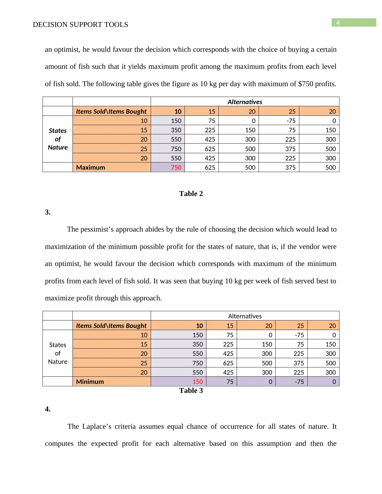
an optimist, he would favour the decision which corresponds with the choice of buying a certain
amount of fish such that it yields maximum profit among the maximum profits from each level
of fish sold. The following table gives the figure as 10 kg per day with maximum of $750 profits.
Alternatives
Items Sold\Items Bought 10 15 20 25 20
States
of
Nature
10 150 75 0 -75 0
15 350 225 150 75 150
20 550 425 300 225 300
25 750 625 500 375 500
20 550 425 300 225 300
Maximum 750 625 500 375 500
Table 2
3.
The pessimist’s approach abides by the rule of choosing the decision which would lead to
maximization of the minimum possible profit for the states of nature, that is, if the vendor were
an optimist, he would favour the decision which corresponds with maximum of the minimum
profits from each level of fish sold. It was seen that buying 10 kg per week of fish served best to
maximize profit through this approach.
Alternatives
Items Sold\Items Bought 10 15 20 25 20
States
of
Nature
10 150 75 0 -75 0
15 350 225 150 75 150
20 550 425 300 225 300
25 750 625 500 375 500
20 550 425 300 225 300
Minimum 150 75 0 -75 0
Table 3
4.
The Laplace’s criteria assumes equal chance of occurrence for all states of nature. It
computes the expected profit for each alternative based on this assumption and then the
5DECISION SUPPORT TOOLS
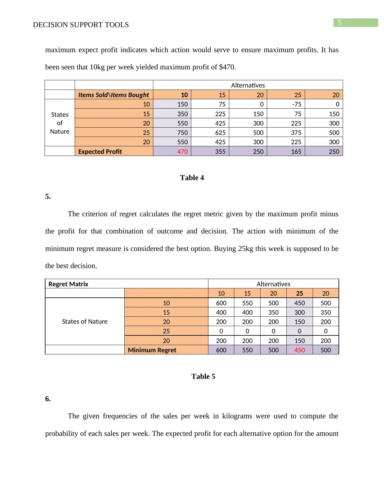
maximum expect profit indicates which action would serve to ensure maximum profits. It has
been seen that 10kg per week yielded maximum profit of $470.
Alternatives
Items Sold\Items Bought 10 15 20 25 20
States
of
Nature
10 150 75 0 -75 0
15 350 225 150 75 150
20 550 425 300 225 300
25 750 625 500 375 500
20 550 425 300 225 300
Expected Profit 470 355 250 165 250
Table 4
5.
The criterion of regret calculates the regret metric given by the maximum profit minus
the profit for that combination of outcome and decision. The action with minimum of the
minimum regret measure is considered the best option. Buying 25kg this week is supposed to be
the best decision.
Regret Matrix Alternatives
10 15 20 25 20
States of Nature
10 600 550 500 450 500
15 400 400 350 300 350
20 200 200 200 150 200
25 0 0 0 0 0
20 200 200 200 150 200
Minimum Regret 600 550 500 450 500
Table 5
6.
The given frequencies of the sales per week in kilograms were used to compute the
probability of each sales per week. The expected profit for each alternative option for the amount
⊘ This is a preview!⊘
Do you want full access?
Subscribe today to unlock all pages.
Trusted by 1+ million students worldwide
6DECISION SUPPORT TOOLS
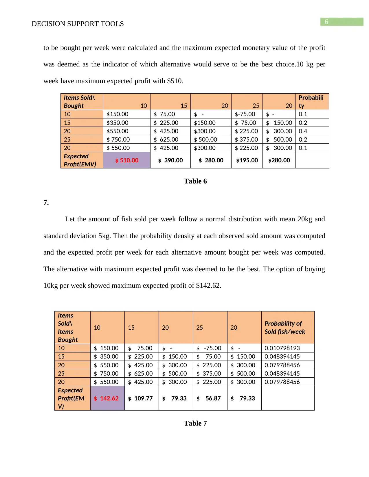
to be bought per week were calculated and the maximum expected monetary value of the profit
was deemed as the indicator of which alternative would serve to be the best choice.10 kg per
week have maximum expected profit with $510.
Items Sold\
Bought 10 15 20 25 20
Probabili
ty
10 $150.00 $ 75.00 $ - $-75.00 $ - 0.1
15 $350.00 $ 225.00 $150.00 $ 75.00 $ 150.00 0.2
20 $550.00 $ 425.00 $300.00 $ 225.00 $ 300.00 0.4
25 $ 750.00 $ 625.00 $ 500.00 $ 375.00 $ 500.00 0.2
20 $ 550.00 $ 425.00 $300.00 $ 225.00 $ 300.00 0.1
Expected
Profit(EMV) $ 510.00 $ 390.00 $ 280.00 $195.00 $280.00
Table 6
7.
Let the amount of fish sold per week follow a normal distribution with mean 20kg and
standard deviation 5kg. Then the probability density at each observed sold amount was computed
and the expected profit per week for each alternative amount bought per week was computed.
The alternative with maximum expected profit was deemed to be the best. The option of buying
10kg per week showed maximum expected profit of $142.62.
Items
Sold\
Items
Bought
10 15 20 25 20 Probability of
Sold fish/week
10 $ 150.00 $ 75.00 $ - $ -75.00 $ - 0.010798193
15 $ 350.00 $ 225.00 $ 150.00 $ 75.00 $ 150.00 0.048394145
20 $ 550.00 $ 425.00 $ 300.00 $ 225.00 $ 300.00 0.079788456
25 $ 750.00 $ 625.00 $ 500.00 $ 375.00 $ 500.00 0.048394145
20 $ 550.00 $ 425.00 $ 300.00 $ 225.00 $ 300.00 0.079788456
Expected
Profit(EM
V)
$ 142.62 $ 109.77 $ 79.33 $ 56.87 $ 79.33
Table 7
Paraphrase This Document
Need a fresh take? Get an instant paraphrase of this document with our AI Paraphraser
7DECISION SUPPORT TOOLS
Question 2.
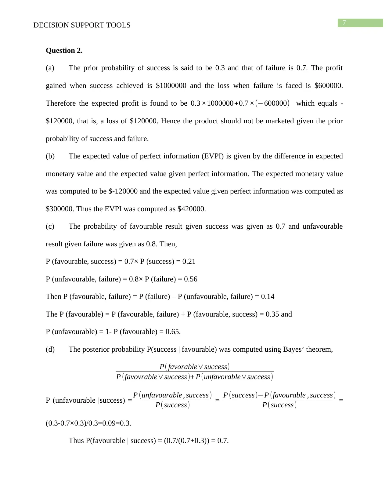
(a) The prior probability of success is said to be 0.3 and that of failure is 0.7. The profit
gained when success achieved is $1000000 and the loss when failure is faced is $600000.
Therefore the expected profit is found to be 0.3 ×1000000+0.7 ×(−600000) which equals -
$120000, that is, a loss of $120000. Hence the product should not be marketed given the prior
probability of success and failure.
(b) The expected value of perfect information (EVPI) is given by the difference in expected
monetary value and the expected value given perfect information. The expected monetary value
was computed to be $-120000 and the expected value given perfect information was computed as
$300000. Thus the EVPI was computed as $420000.
(c) The probability of favourable result given success was given as 0.7 and unfavourable
result given failure was given as 0.8. Then,
P (favourable, success) = 0.7× P (success) = 0.21
P (unfavourable, failure) = 0.8× P (failure) = 0.56
Then P (favourable, failure) = P (failure) – P (unfavourable, failure) = 0.14
The P (favourable) = P (favourable, failure) + P (favourable, success) = 0.35 and
P (unfavourable) = 1- P (favourable) = 0.65.
(d) The posterior probability P(success | favourable) was computed using Bayes’ theorem,
P( favorable∨success)
P (favovrable∨success)+ P(unfavorable∨success)
P (unfavourable |success) = P (unfavourable , success)
P( success) = P (success)−P (favourable , success)
P(success) =
(0.3-0.7×0.3)/0.3=0.09=0.3.
Thus P(favourable | success) = (0.7/(0.7+0.3)) = 0.7.
Question 2.
(a) The prior probability of success is said to be 0.3 and that of failure is 0.7. The profit
gained when success achieved is $1000000 and the loss when failure is faced is $600000.
Therefore the expected profit is found to be 0.3 ×1000000+0.7 ×(−600000) which equals -
$120000, that is, a loss of $120000. Hence the product should not be marketed given the prior
probability of success and failure.
(b) The expected value of perfect information (EVPI) is given by the difference in expected
monetary value and the expected value given perfect information. The expected monetary value
was computed to be $-120000 and the expected value given perfect information was computed as
$300000. Thus the EVPI was computed as $420000.
(c) The probability of favourable result given success was given as 0.7 and unfavourable
result given failure was given as 0.8. Then,
P (favourable, success) = 0.7× P (success) = 0.21
P (unfavourable, failure) = 0.8× P (failure) = 0.56
Then P (favourable, failure) = P (failure) – P (unfavourable, failure) = 0.14
The P (favourable) = P (favourable, failure) + P (favourable, success) = 0.35 and
P (unfavourable) = 1- P (favourable) = 0.65.
(d) The posterior probability P(success | favourable) was computed using Bayes’ theorem,
P( favorable∨success)
P (favovrable∨success)+ P(unfavorable∨success)
P (unfavourable |success) = P (unfavourable , success)
P( success) = P (success)−P (favourable , success)
P(success) =
(0.3-0.7×0.3)/0.3=0.09=0.3.
Thus P(favourable | success) = (0.7/(0.7+0.3)) = 0.7.
8DECISION SUPPORT TOOLS
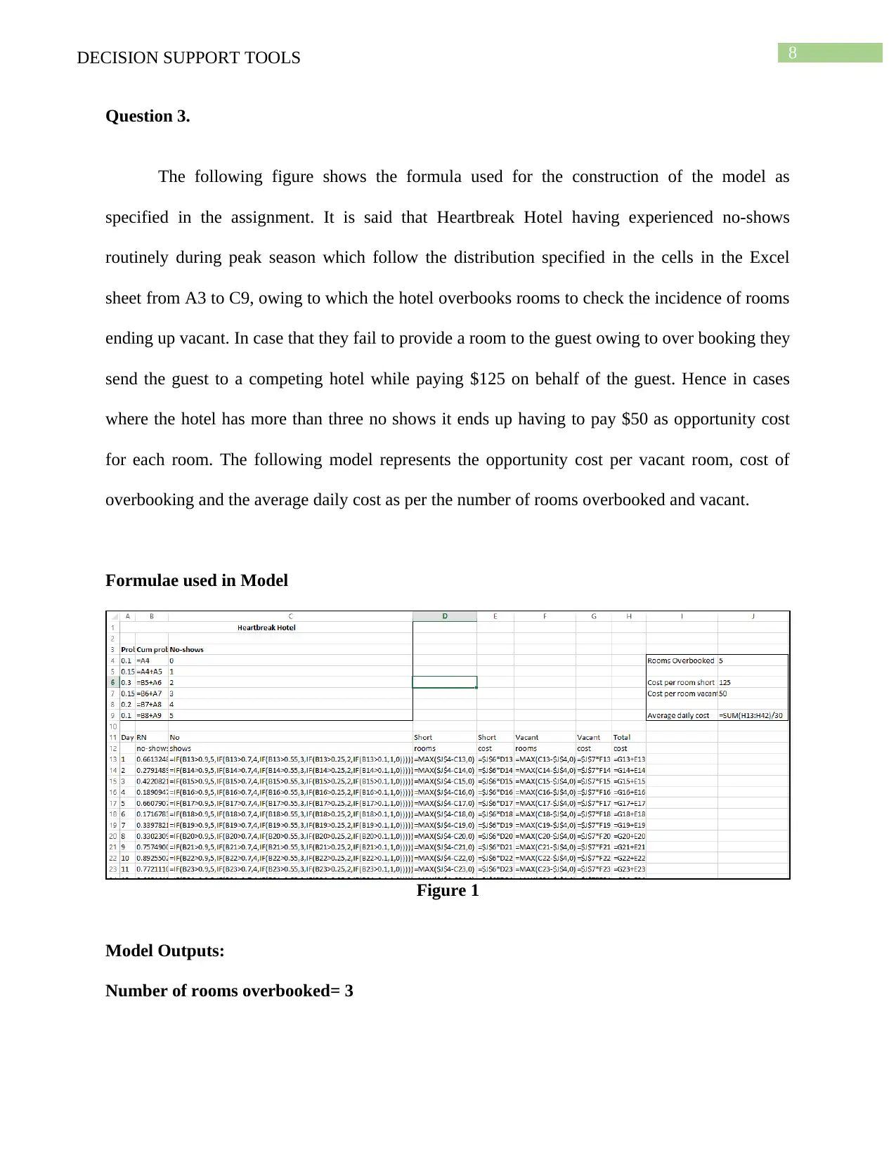
Question 3.
The following figure shows the formula used for the construction of the model as
specified in the assignment. It is said that Heartbreak Hotel having experienced no-shows
routinely during peak season which follow the distribution specified in the cells in the Excel
sheet from A3 to C9, owing to which the hotel overbooks rooms to check the incidence of rooms
ending up vacant. In case that they fail to provide a room to the guest owing to over booking they
send the guest to a competing hotel while paying $125 on behalf of the guest. Hence in cases
where the hotel has more than three no shows it ends up having to pay $50 as opportunity cost
for each room. The following model represents the opportunity cost per vacant room, cost of
overbooking and the average daily cost as per the number of rooms overbooked and vacant.
Formulae used in Model
Figure 1
Model Outputs:
Number of rooms overbooked= 3
⊘ This is a preview!⊘
Do you want full access?
Subscribe today to unlock all pages.
Trusted by 1+ million students worldwide
9DECISION SUPPORT TOOLS
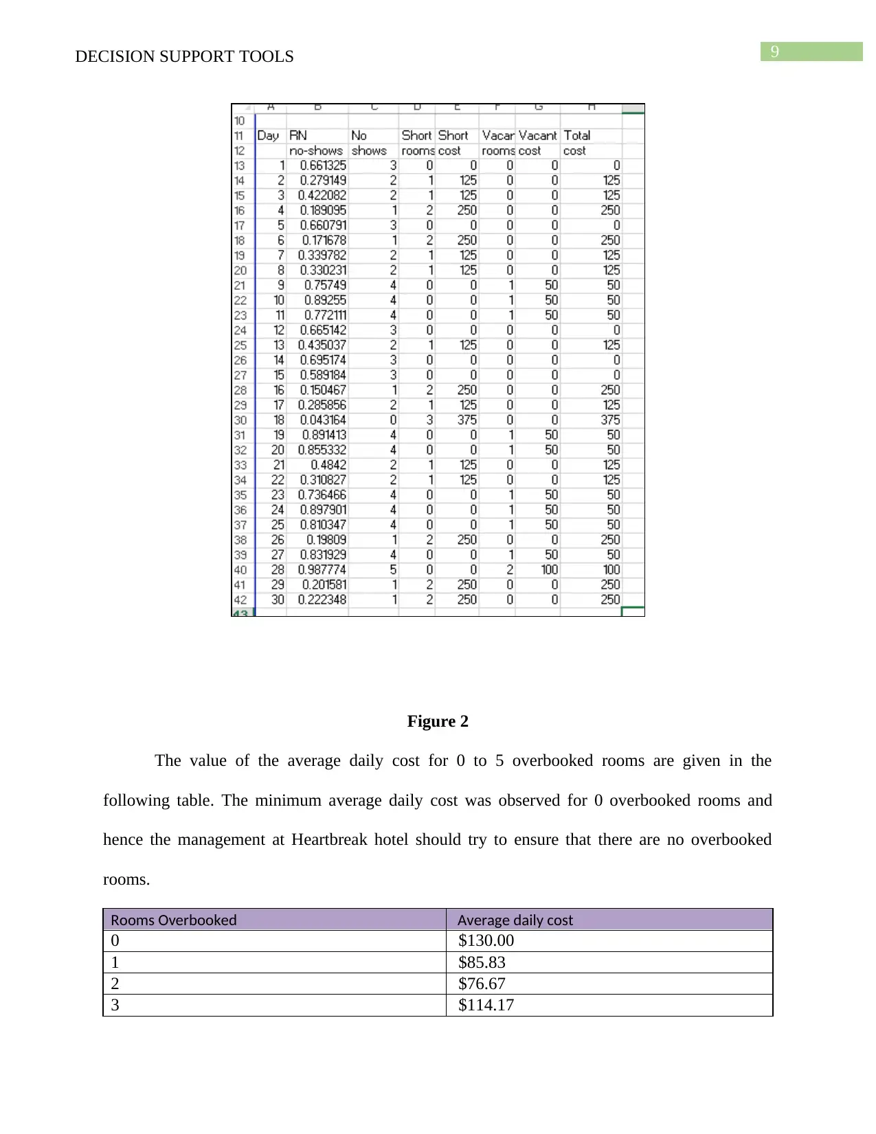
Figure 2
The value of the average daily cost for 0 to 5 overbooked rooms are given in the
following table. The minimum average daily cost was observed for 0 overbooked rooms and
hence the management at Heartbreak hotel should try to ensure that there are no overbooked
rooms.
Rooms Overbooked Average daily cost
0 $130.00
1 $85.83
2 $76.67
3 $114.17
Paraphrase This Document
Need a fresh take? Get an instant paraphrase of this document with our AI Paraphraser
10DECISION SUPPORT TOOLS
4 $180.83
5 $300.00
Table 8
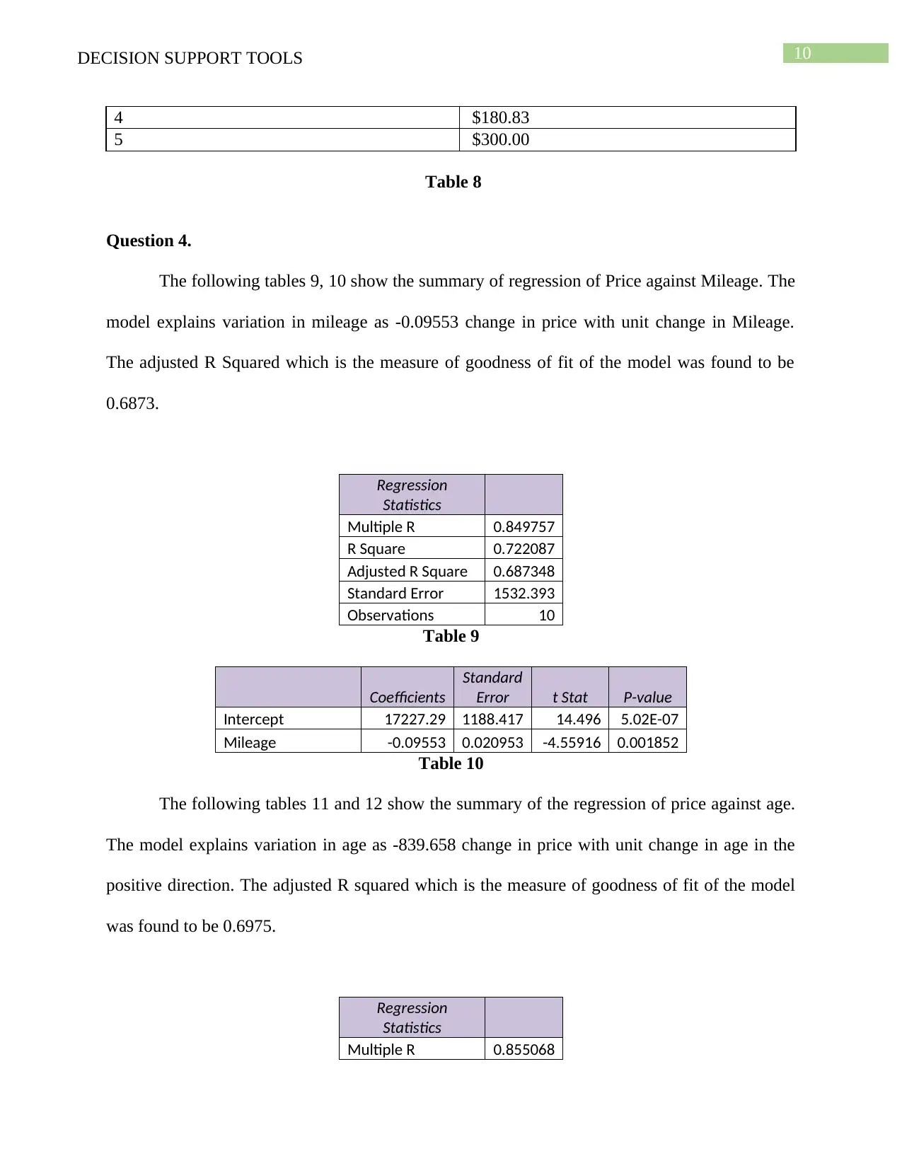
Question 4.
The following tables 9, 10 show the summary of regression of Price against Mileage. The
model explains variation in mileage as -0.09553 change in price with unit change in Mileage.
The adjusted R Squared which is the measure of goodness of fit of the model was found to be
0.6873.
Regression
Statistics
Multiple R 0.849757
R Square 0.722087
Adjusted R Square 0.687348
Standard Error 1532.393
Observations 10
Table 9
Coefficients
Standard
Error t Stat P-value
Intercept 17227.29 1188.417 14.496 5.02E-07
Mileage -0.09553 0.020953 -4.55916 0.001852
Table 10
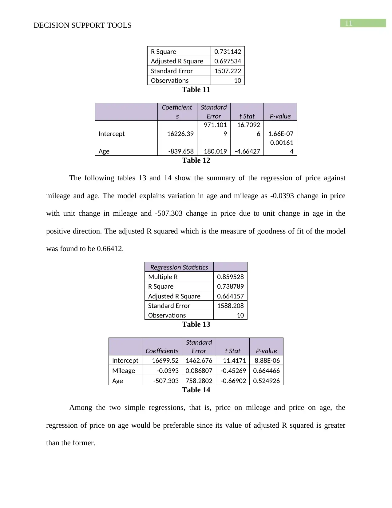
The following tables 11 and 12 show the summary of the regression of price against age.
The model explains variation in age as -839.658 change in price with unit change in age in the
positive direction. The adjusted R squared which is the measure of goodness of fit of the model
was found to be 0.6975.
Regression
Statistics
Multiple R 0.855068
4 $180.83
5 $300.00
Table 8
Question 4.
The following tables 9, 10 show the summary of regression of Price against Mileage. The
model explains variation in mileage as -0.09553 change in price with unit change in Mileage.
The adjusted R Squared which is the measure of goodness of fit of the model was found to be
0.6873.
Regression
Statistics
Multiple R 0.849757
R Square 0.722087
Adjusted R Square 0.687348
Standard Error 1532.393
Observations 10
Table 9
Coefficients
Standard
Error t Stat P-value
Intercept 17227.29 1188.417 14.496 5.02E-07
Mileage -0.09553 0.020953 -4.55916 0.001852
Table 10
The following tables 11 and 12 show the summary of the regression of price against age.
The model explains variation in age as -839.658 change in price with unit change in age in the
positive direction. The adjusted R squared which is the measure of goodness of fit of the model
was found to be 0.6975.
Regression
Statistics
Multiple R 0.855068
11DECISION SUPPORT TOOLS
R Square 0.731142
Adjusted R Square 0.697534
Standard Error 1507.222
Observations 10
Table 11
Coefficient
s
Standard
Error t Stat P-value
Intercept 16226.39
971.101
9
16.7092
6 1.66E-07
Age -839.658 180.019 -4.66427
0.00161
4
Table 12
The following tables 13 and 14 show the summary of the regression of price against
mileage and age. The model explains variation in age and mileage as -0.0393 change in price
with unit change in mileage and -507.303 change in price due to unit change in age in the
positive direction. The adjusted R squared which is the measure of goodness of fit of the model
was found to be 0.66412.
Regression Statistics
Multiple R 0.859528
R Square 0.738789
Adjusted R Square 0.664157
Standard Error 1588.208
Observations 10
Table 13
Coefficients
Standard
Error t Stat P-value
Intercept 16699.52 1462.676 11.4171 8.88E-06
Mileage -0.0393 0.086807 -0.45269 0.664466
Age -507.303 758.2802 -0.66902 0.524926
Table 14
Among the two simple regressions, that is, price on mileage and price on age, the
regression of price on age would be preferable since its value of adjusted R squared is greater
than the former.
⊘ This is a preview!⊘
Do you want full access?
Subscribe today to unlock all pages.
Trusted by 1+ million students worldwide
1 out of 14
Related Documents


![Accounting Decision Support Tools Assessment Item 3 Solution [Date]](/_next/image/?url=https%3A%2F%2Fdesklib.com%2Fmedia%2Fimages%2Fwx%2F8b0579db5dc54829a8e805e0dcb6f432.jpg&w=256&q=75)


![Assignment: Accounting Decision Support Tools - [Date] - Finance](/_next/image/?url=https%3A%2F%2Fdesklib.com%2Fmedia%2Fimages%2Fga%2F85e3fe63d61d4af3a506409b3f137201.jpg&w=256&q=75)
Your All-in-One AI-Powered Toolkit for Academic Success.
+13062052269
info@desklib.com
Available 24*7 on WhatsApp / Email
![[object Object]](/_next/static/media/star-bottom.7253800d.svg)
Unlock your academic potential
Copyright © 2020–2026 A2Z Services. All Rights Reserved. Developed and managed by ZUCOL.