Decision Sciences: Statistical Decision Making and Data Analysis
VerifiedAdded on 2023/06/11
|10
|1977
|171
Homework Assignment
AI Summary
This document provides solutions to a Decision Sciences homework assignment, covering a range of topics including Expected Monetary Value (EMV) analysis, linear programming, and regression analysis. The EMV section explores decision-making under uncertainty, calculating expected values for different scenarios involving hiring nurses and upgrading facilities. The linear programming section focuses on optimizing inventory sales to meet capital requirements, while the regression analysis section examines the relationship between various factors and insurance claims using multiple regression models. Additionally, the assignment tackles probability calculations related to noise levels and penalty payments, as well as decision variables for course selection and track specialization. The solutions demonstrate the application of statistical and optimization techniques to solve real-world problems in business and management.
Running head: DECISION SCIENCES
Decision Sciences
Name of Student:
Name of University:
Course ID:
Decision Sciences
Name of Student:
Name of University:
Course ID:
Paraphrase This Document
Need a fresh take? Get an instant paraphrase of this document with our AI Paraphraser
1DECISION SCIENCES
Table of Contents
Answer 1..........................................................................................................................................2
Part 1:..........................................................................................................................................2
Part 2:..........................................................................................................................................3
Problem 2.........................................................................................................................................6
Problem 3.........................................................................................................................................6
Problem 4.........................................................................................................................................8
Problem 5.........................................................................................................................................9
2DECISION SCIENCES
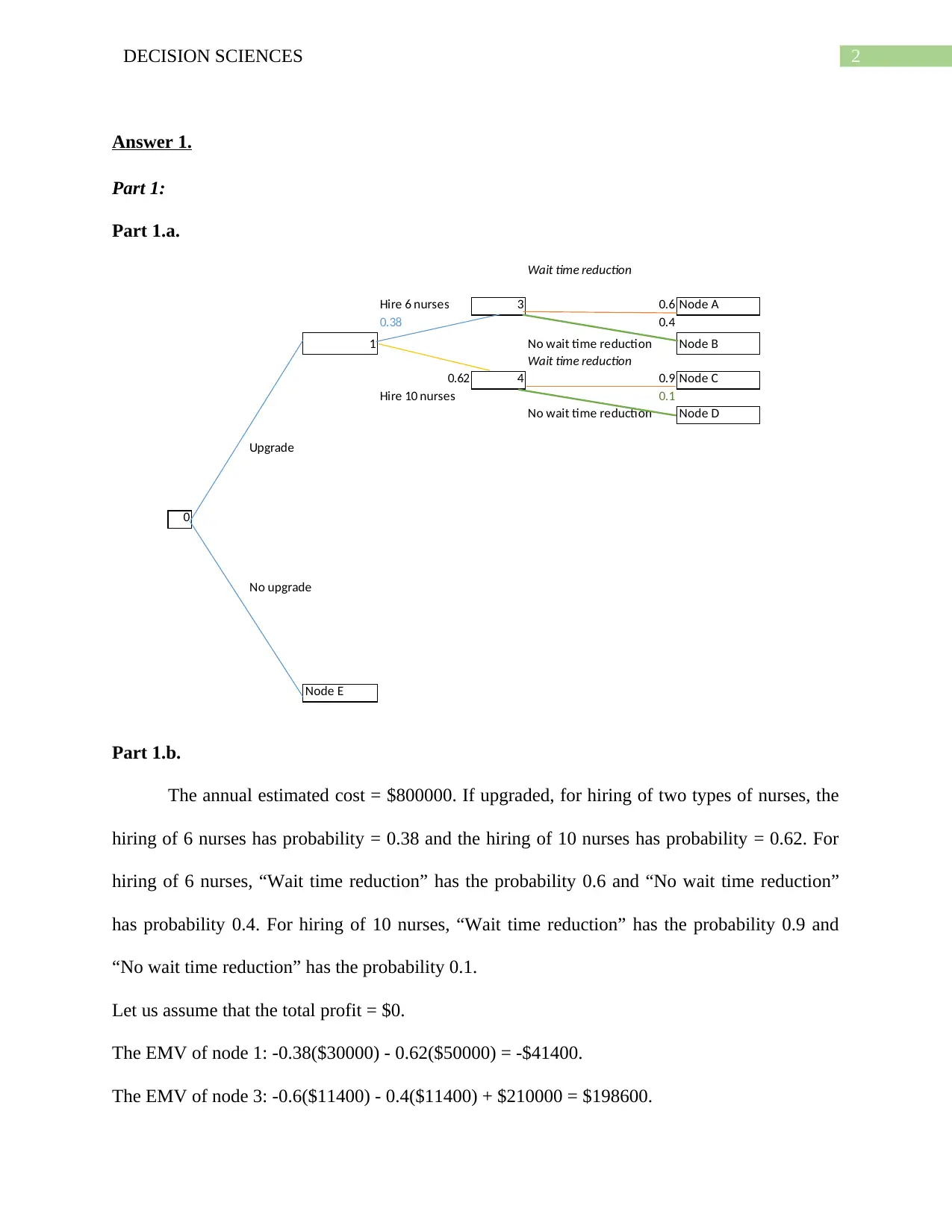
Answer 1.
Part 1:
Part 1.a.
Wait time reduction
Hire 6 nurses 3 0.6 Node A
0.38 0.4
1 No wait time reduction Node B
Wait time reduction
0.62 4 0.9 Node C
Hire 10 nurses 0.1
No wait time reduction Node D
Upgrade
0
No upgrade
Node E
Part 1.b.
The annual estimated cost = $800000. If upgraded, for hiring of two types of nurses, the
hiring of 6 nurses has probability = 0.38 and the hiring of 10 nurses has probability = 0.62. For
hiring of 6 nurses, “Wait time reduction” has the probability 0.6 and “No wait time reduction”
has probability 0.4. For hiring of 10 nurses, “Wait time reduction” has the probability 0.9 and
“No wait time reduction” has the probability 0.1.
Let us assume that the total profit = $0.
The EMV of node 1: -0.38($30000) - 0.62($50000) = -$41400.
The EMV of node 3: -0.6($11400) - 0.4($11400) + $210000 = $198600.
⊘ This is a preview!⊘
Do you want full access?
Subscribe today to unlock all pages.
Trusted by 1+ million students worldwide
3DECISION SCIENCES
The EMV of node 4: -0.9($31000) - 0.1($31000) + $210000 = $180000.
The EMV of node A: -0.6($11400) = -$68400.
The EMV of node B: -0.4($11400) = -$45600.
The EMV of node C: -0.9($31000) = -$27900.
The EMV of node D: -0.1($31000) = -$3100.
The EMV of node E: -$80000+($30000 + $50000) = $0.0.
Part 1.c.
The decision tree has branches and leaves to predictive nature of variables on various
considerations. The questions shown in decision tree follows a step by step format in which
questions cited in recursive relation provides the answers sequentially. As, the popular technique
“Simulation” can be more confusing because decisions are modelled as rules and used with
general statistical distributions whereas a decision tree assesses the probability value and could
be visualized with the help of a tree. Decision tree goes with “Strategy map” for decisions and
values going forward. Expected Monetary Value (EMV) is a recommended tool and techniques
for project risk management. The accounting office has computed a loss of more than $1200000
relative to the old situation as high risky.
Part 2:
a) X ~ Bin (30, 0.5).
P (X =3) = 30 !
3! 27! . (0.5)3 (1-0.5) (30-3) = 30∗29∗28
6 ∗( 0.5 )30
= 0.00000378.
Hence, P (X = 3) lies in the range of 0 to 0.2.
b)
Paraphrase This Document
Need a fresh take? Get an instant paraphrase of this document with our AI Paraphraser
4DECISION SCIENCES
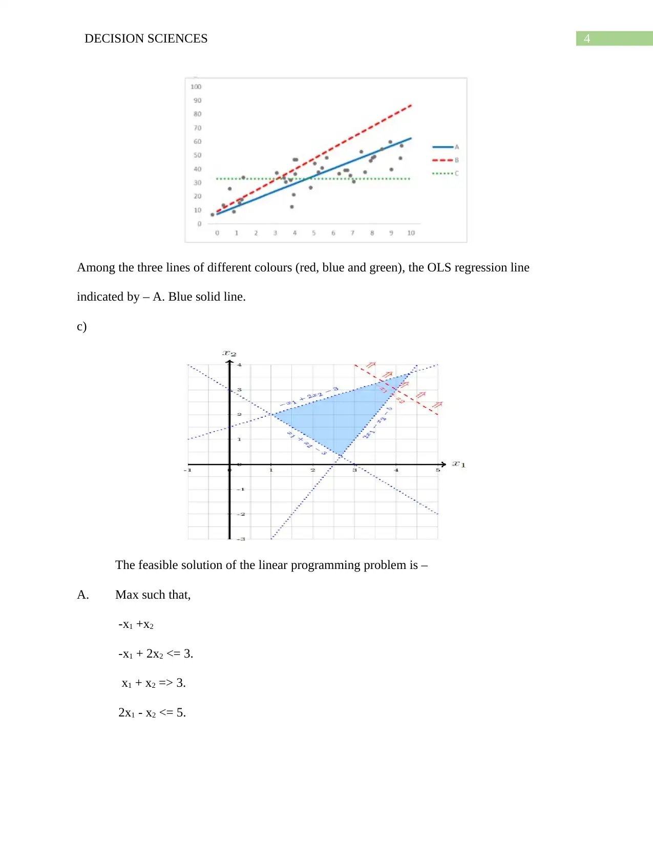
Among the three lines of different colours (red, blue and green), the OLS regression line
indicated by – A. Blue solid line.
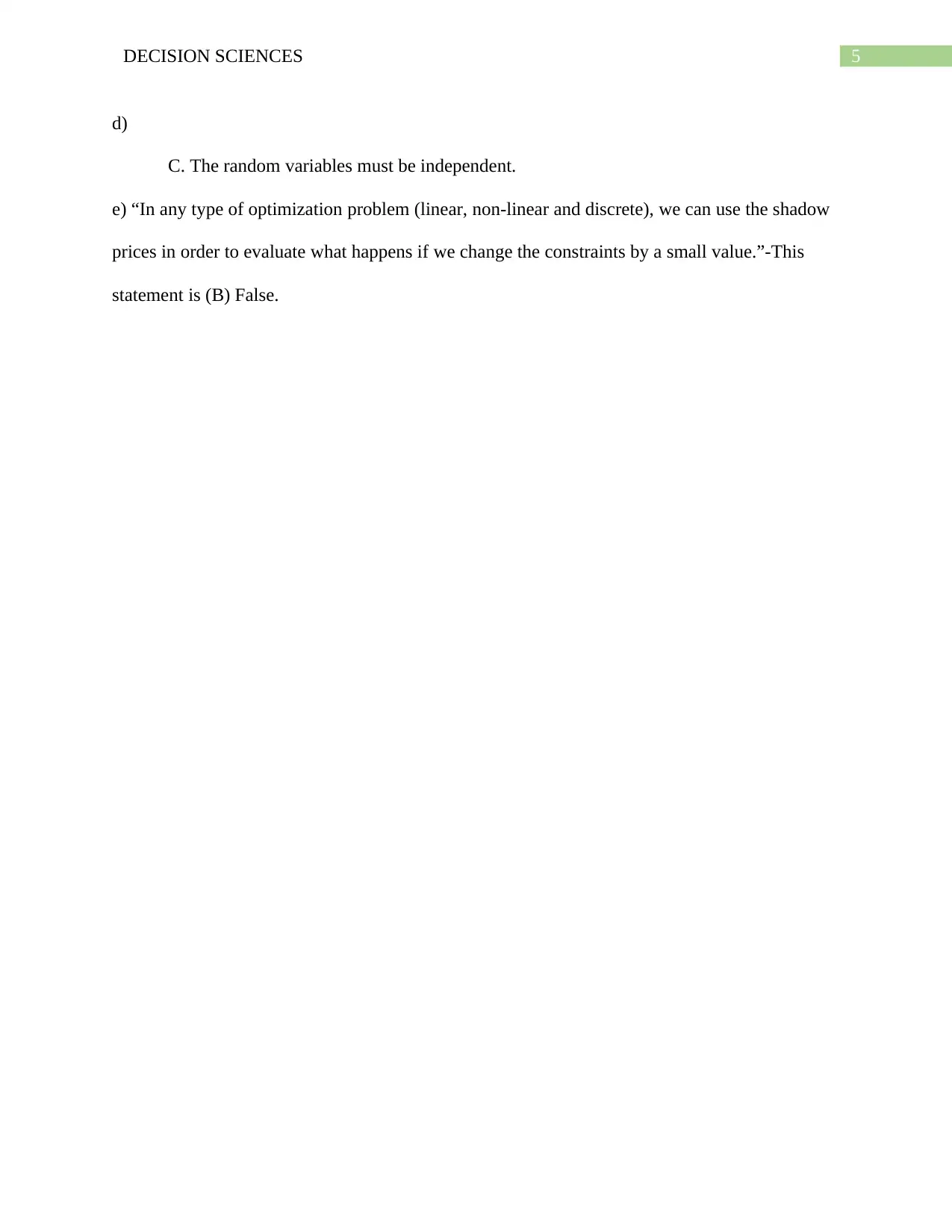
c)
The feasible solution of the linear programming problem is –
A. Max such that,
-x1 +x2
-x1 + 2x2 <= 3.
x1 + x2 => 3.
2x1 - x2 <= 5.
Among the three lines of different colours (red, blue and green), the OLS regression line
indicated by – A. Blue solid line.
c)
The feasible solution of the linear programming problem is –
A. Max such that,
-x1 +x2
-x1 + 2x2 <= 3.
x1 + x2 => 3.
2x1 - x2 <= 5.
5DECISION SCIENCES
d)
C. The random variables must be independent.
e) “In any type of optimization problem (linear, non-linear and discrete), we can use the shadow
prices in order to evaluate what happens if we change the constraints by a small value.”-This
statement is (B) False.
d)
C. The random variables must be independent.
e) “In any type of optimization problem (linear, non-linear and discrete), we can use the shadow
prices in order to evaluate what happens if we change the constraints by a small value.”-This
statement is (B) False.
⊘ This is a preview!⊘
Do you want full access?
Subscribe today to unlock all pages.
Trusted by 1+ million students worldwide
6DECISION SCIENCES
Problem 2.
a) The objective function of the model is given as-
15000 = 300*Inventory A + 800*Inventory B+ 150*Inventory C
b) The constraint amount raised from selling inventory should be at least $15,000 is given as-
300*Inventory A + 757.143*Inventory B + 150*Inventory C ≥ 15000.
c) The optimal quantities of inventories that Mitchela needs to put on sale to meet her capital
requirement of $15,000 is 300 for inventory A, 42.857 for Inventory B and 0 for Inventory C.
d) The allowable increase to the constraint of inventory of product B (1E+30) is 7.5 units.
e) Mitchela is told that the new magnets she is planning to order would cost $19,000 in
replacement of $15,000. With regard to this, Mitchela is going to have to put even more current
inventory on sale.
The new optimal expected value of the leftover inventory for next week would be –
375 * inventory A + 800 * Inventory B + 150 * Inventory C ≥ 19000.
The allowable increase of the constraint corresponding to the $D$27 is $53000. It means that,
under provided constraints (Inventory A = 75, Inventory B = 1E+30 and Inventory C = 1E+30),
the valuation of the optimised solution could be $53000.
Problem 3.
a) As per model 1, the multiple regression model is given by-
“Claims” = 23.327 – 3.011* “District” – 9.124* “Age<25” – 6.226* “Age 25-29” – 7.666* “Age
30-35” + 0.107* “Holders”.
b) The 95% upper and lower confidence intervals of the variable “District” are-
Upper CI of District = (-3.010634313) + TINV(0.05, 58) * 1.462858948 = (-0.0824).
Paraphrase This Document
Need a fresh take? Get an instant paraphrase of this document with our AI Paraphraser
7DECISION SCIENCES
Lower CI of District = (-3.010634313) - TINV(0.05, 58) * 1.462858948 = (-5.93886).
c) The p-values calculated by the formula (TDIST(ABS(t-stat), df of residuals, 2)) for each
variable indicate that-
District (p-value = 0.044089) has p-value less than 5%. Hence, the variable has linear
significant effect on the dependent variable “Claims”.
“Age<25” (p-value = 0.09755) has p-value greater than 5%. Hence, the variable does not
have linear significant effect on the dependent variable “Claims”.
“Age 25-29” (p-value = 0.241167) has p-value greater than 5%. Therefore, the variable
does not have linear significant effect on the dependent variable “Claims”.
“Age 30-35” (p-value = 0.143628) has p-value greater than 5%. Hence, the variable does
not have linear significant effect on the dependent variable “Claims”.
“Holders” (p-value = 0.00000) has p-value less than 5%. Hence, the variable has linear
significant effect on the dependent variable “Claims”.
d) The coefficient of the predictor “Holders” in this regression model is 0.1073705. It signifies a
positive relationship between “Holders” and “Claims’. For 1 unit increase or decrease of holders,
the claiming amount also increases or decreases by 0.1073705 unit.
e) Tamar must prefer model 2 rather than model 1. The values of R-square are almost equal in
both the model. Hence, the models are almost equally important with respect to their explanatory
power. The first model only considers two significant predictors along with 3 insignificant
predictors, whereas the second model only considers 1 significant factor. Holder is alone enough
strong to describe a significant association with claims. The t-values in the first model was very
low and negative in the first model and the t-value of Holder in the second model is higher than
8DECISION SCIENCES
the first model. Hence, from this angle too, Tamar would show his sensibility to choose the
model 2.
f) Both the linear regression models (model 1 and model 2) explains more than 90% variability
of the dependent variable. Hence, linear regression model is a good choice to explain the
variability of claims and predict the dependent variable claims. Non-linear transformations such
as log transformation may be a better option; however, the non-linear transformation of the
variables is not necessary.
g) The linear regression model is given as-
“Claims” = 8.122017843 + 0.112641417 * ‘Holders”.
As per second regression model, claim = 8.122017843 + 0.11261417 * 212 = 31.996 ≈32.
The probability that a group of 212 policyholders living in a minor town below the age of 25
would make more than 50 claims as per model 2 is – (1 - 32
50 ¿=0.36 .
Problem 4.
a) The probability that at least 5 days out of next 7 days would have noise levels within the
threshold is –
Bin (5,7, 0.9) = 7 !
5! 2 ! . (0.9)5. (0.1)(7-5) + 7 !
6 ! 1! . (0.9)6. (0.1)(7-6) + 7 !
7 ! 0 !. (0.9)7. (0.1)(7-7) = 0.124+
0.372+0.4783 = 0.9743. [ p = 0.9, q = 0.1, n = 7, r = 5(1)7].
b) The distribution of Z is Normal.
Z denote the total penalty payment that the construction company would have to pay to the
MIT administration. Its mean = n*p = $30*(1000*0.1) = $3000.
⊘ This is a preview!⊘
Do you want full access?
Subscribe today to unlock all pages.
Trusted by 1+ million students worldwide
9DECISION SCIENCES
The standard deviation of the total penalty payment that the construction company would
have to pay to the MIT administration has standard deviation = n*p*q = $30*(1000*0.1*0.9) =
$27000.
c) The probability that the total penalty in the next 30 days is going to be less than $5000 is –
P(Z<5000) = P ( Z−3000
27000 < 5000−3000
27000 ) = P(Z*<0.074074) = 0.5295.
d) The probability that the penalty would be between $2000 and $4000 is –
P(2000<Z<4000) = P ( 2000−3000
27000 < Z∗¿ 4 000−3000
27000 ) = P (-0.037037<Z*<0.037037) = P (Z*<
|0.037037|) = 0.5148.
Problem 5.
1)
a. The set of decision variables that refer that the student takes course c in semester s is given by-
“Average hours/week” and “Elisabeth’s joy”.
b. The set of decision variables that indicate three tracks such as “General Track”, “Analytics
Track” and “operations Management Track” are given below.
1 out of 10
Your All-in-One AI-Powered Toolkit for Academic Success.
+13062052269
info@desklib.com
Available 24*7 on WhatsApp / Email
![[object Object]](/_next/static/media/star-bottom.7253800d.svg)
Unlock your academic potential
Copyright © 2020–2026 A2Z Services. All Rights Reserved. Developed and managed by ZUCOL.