Decision Support Tools: Analysis of Business Decision Making

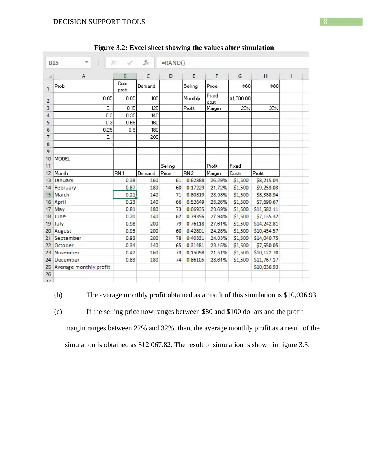
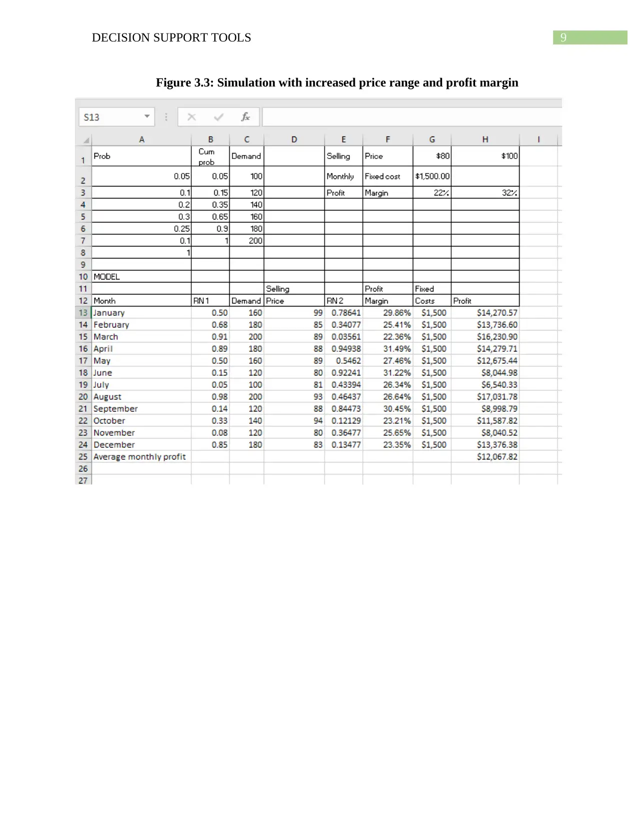
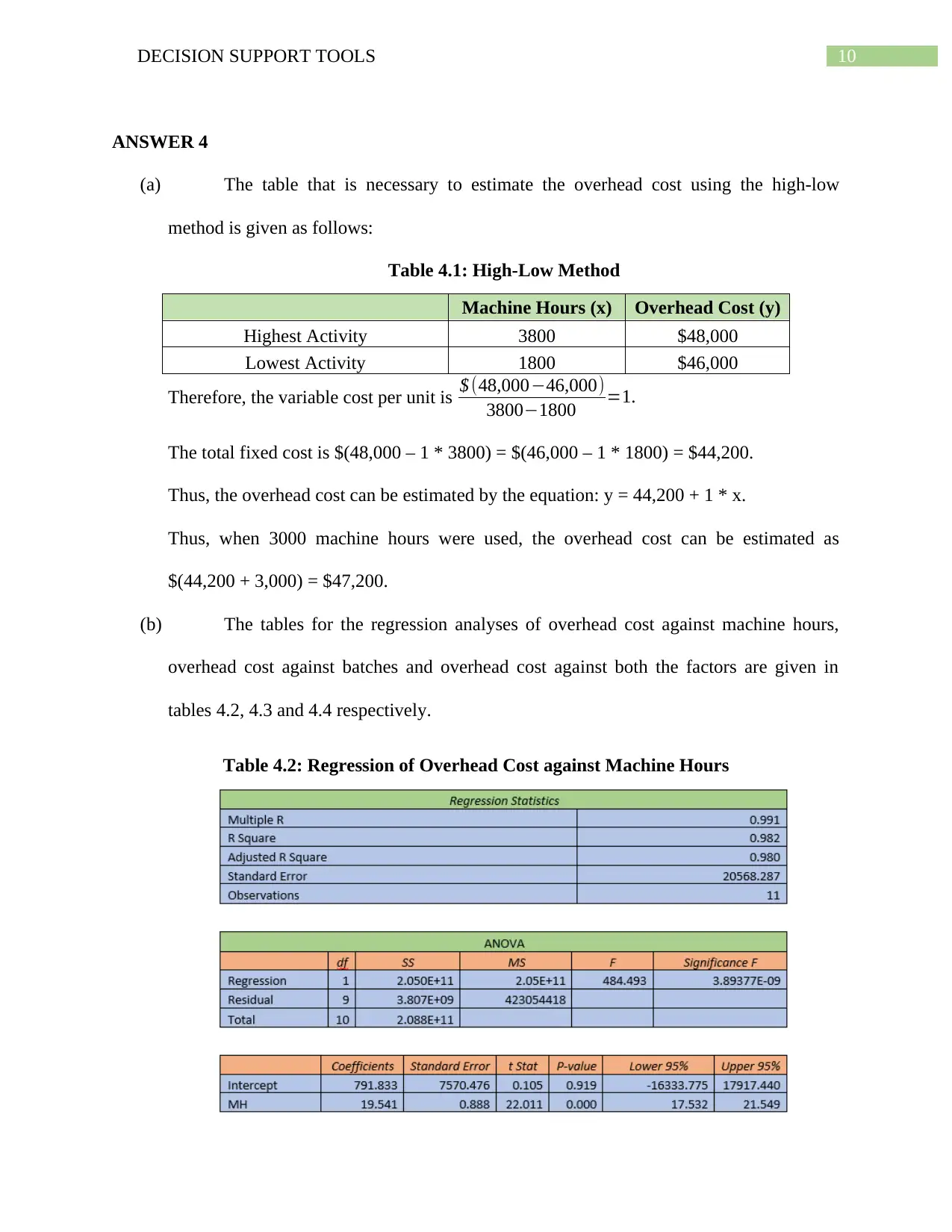
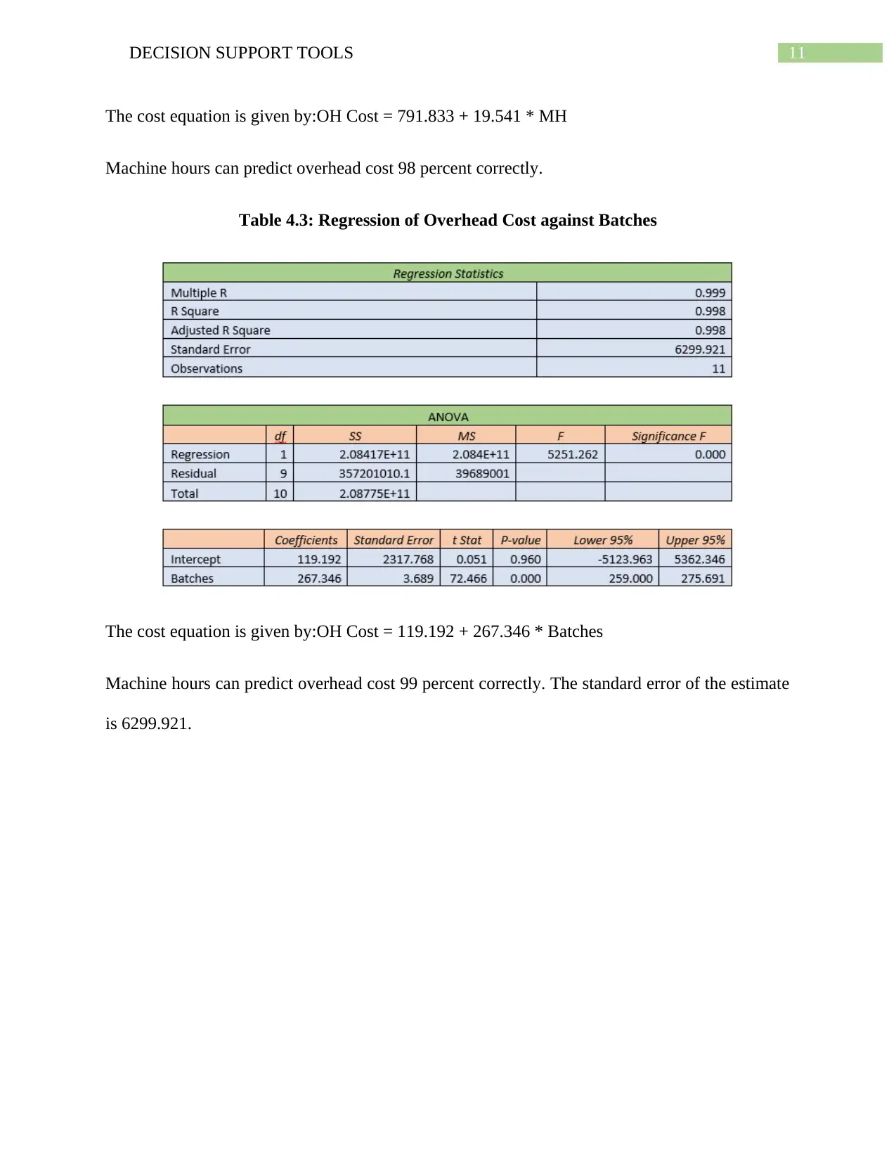
This assignment delves into the application of decision support tools across various business scenarios. It begins by exploring decision-making under certainty, risk, and uncertainty, illustrated through an investment payoff matrix. The solution employs different decision-making criteria such as optimist, pessimist, and regret, alongside expected value calculations to guide investment choices. The assignment then analyzes a bicycle shop scenario, comparing the profitability of large and small shops under different market conditions, incorporating prior and posterior probabilities. Furthermore, it utilizes Excel simulation to determine average monthly profit under varying price ranges and profit margins. The document also presents a high-low method analysis to estimate overhead costs, followed by regression analyses to predict overhead costs using machine hours and batches, concluding with a break-even and profit analysis for product manufacturing, considering different profit targets and product ratios.

Running Head: DECISION SUPPORT TOOLS
Decision Support Tools
Name of the Student
Name of the University
Author Note

1DECISION SUPPORT TOOLS
Table of Contents
ANSWER 1.....................................................................................................................................2
ANSWER 2.....................................................................................................................................5
ANSWER 3.....................................................................................................................................7
ANSWER 4...................................................................................................................................10
ANSWER 5...................................................................................................................................13
BIBLIOGRAPHY..........................................................................................................................15

2DECISION SUPPORT TOOLS
ANSWER 1
(a) A person will be making a decision under certainty if he has all the information
that will be considered in order to make a decision.
A person will be said to be making a decision under risk if all the decision that are
possible to make have a certain probability of occurrence. In this case, the probability of
the decision that the person makes will be considered as the risk of making that decision.
A person will be making a decision under uncertainty if he has incomplete
information or no information about the matter on which the decision has to be made.
(b) Bikram Shrestha inherited some money and he wants to invest that amount in any
of the following markets – Share Market, Bonds or Real Estate. The following payoff
matrix gives the profit figures of the markets for the upcoming year.
Table 1: Payoff Matrix
Good Economy Poor Economy
Share market $80,000 ($20,000)
Bonds 30,000 20,000
Real estate 25,000 15,000
1. The choice of an optimist would be to choose the profit which is
maximum in all respects. In other words, he will choose the alternative where the
maximum payoff is maximized. Table 2 gives the figures for the maximum profit
earned from each of the markets and the choice of the alternative is highlighted.
Thus, the decision of an optimist would be to invest in share markets.

3DECISION SUPPORT TOOLS
Table 2: Optimist’s Choice
Good Economy Poor Economy Best Profit / Loss
Share market $80,000 ($20,000) $80,000
Bonds $30,000 $20,000 $30,000
Real estate $25,000 $15,000 $25,000
2. The choice of a pessimist would be to invest in a market in which the
minimum payoff is maximized. Table 3 shows the least possible profits and the
maximum of the least possible profits are highlighted. It can be seen that the
maximum profit from the minimum payoffs can be earned from bonds. Thus, the
decision of apessimist would be to invest in bonds.
Table 2: Decision of a Pessimist
Good Economy Poor Economy Least Profit / Loss
Share market $80,000 -$20,000.00 -$20,000.00
Bonds $30,000 $20,000.00 $20,000.00
Real estate $25,000 $15,000.00 $15,000.00
3. A criterion of regret is defined as minimizing the maximum regret. Here,
regret indicates opportunity loss. Thus, regret = best payoff – payoff received.
Then, the first table can be framed as follows in terms of regret. The minimum
regret value has been found in Share market as seen from table 4. Thus, the
decision should be to invest in share markets.
Table 4: Table of Regret
Good Economy Poor Economy Maximum
Share market $0 $40,000.00 $40,000.00
Bonds $50,000 $0.00 $50,000.00
Real estate $55,000 $5,000.00 $55,000.00
4. According to the question, the probability of a good economy is 0.3. Thus,
the probability of a poor economy is (1 – 0.3) = 0.7.
Therefore, the expected profits in
Share Market = (0.3 * $80,000) – (0.7 * $20,000) = $10,000.

4DECISION SUPPORT TOOLS
Bonds = (0.3 * $30,000) + (0.7 * $20,000) = $23,000.
Real Estate = (0.3 * $25,000) – (0.7 * $15,000) = $18,000.
Thus, from the above calculations, it is evident that investing in bonds will
be the optimum action.
5. The expected value of perfect information (EVPI) is given by the formula
EVPI=∑
j
p j ( max
i Aij )−max
i ∑
j
p j Aij, where, Aij is the value of the ith row and jth
column and pj is the probability of that cell.
Thus, ∑
j
p j ( max
i Aij ) = (0.3 * $80,000) + (0.3 * $30,000) + (0.3 * $25,000) =
$40,500.
Again, max
i ∑
j
p j Aij=¿$23,000.
Therefore, EVPI = $(40,500 – 23000) = $17,500.

5DECISION SUPPORT TOOLS
ANSWER 2
(a) Jerry wants to open a bicycle shop. He can open two types of shops – large shops
(a1) and small shops (a2). There are two types of markets – good market (s1) and poor
market (s2). According to his beliefs, in a large shop, there will be a profit of $80,000 in a
good market and a loss of $40,000 in a poor market. There is a 50 percent chance for the
market to be good or bad. Thus, in a large shop, the estimated profit will be:
P (a1) = $80,000 * P (s1) + $(- 40,000) * P (s2)
= $(80,000 * 0.5 – 40,000 * 0.5)
= $20,000.
In a small shop, jerry believes that there will be a profit of $30,000 in a good
market and a loss of $10,000 in a poor market.Thus, in a small shop, the estimated profit
will be:
P (a2) = $30,000 * P (s1) + $(- 10,000) * P (s2)
= $(30,000 * 0.5 – 10,000 * 0.5)
= $10,000.
Thus, whether the market is good or bad, profit is more in a large shop compared
to a small shop. Thus, Jerry should open a large shop.
(b) Jerry appointed a friend who provided a track record. According to the record the
previous probabilities has been revised. Let A denote a favorable market and B denote an
unfavorable market. It has been assumed that in both the good and poor market
conditions, there has been no profit or loss in an unfavorable market. Thus, in a large
shop, the revised prior probability will be:
P (a1) = P (s1) * P (A) + P (s2) * P (B)

6DECISION SUPPORT TOOLS
= 0.5 * 0.8 + 0.5 * 0.2
= 0.5.
Thus, in a small shop, the revised prior probability will be:
P (a2) = P (s1) * P (A) + P (s2) * P (B)
= 0.5 * 0.8 + 0.5 * 0.4
= 0.5.
(c) The posterior probability of a good market given that his friend has provided an
unfavorable market prediction is P (s1) * P (B) = 0.5 * 0.2 = 0.1.
(d) The expected net gain in a large market is
P (a1) = $80,000 * P (s1) * P (A) + $(- 40,000) * P (s2) * P (B)
= $(80,000 * 0.5 * 0.8 – 40,000 * 0.5 * 0.2)
= $24,000.
The expected gain in small market is
P (a2) = $30,000 * P (s1) * P (A) + $(- 10,000) * P (s2) * P (B)
= $(30,000 * 0.5 * 0.8 – 10,000 * 0.5 * 0.2)
= $10,000.
If his friend is engaged to conduct the market research, the profit in the large
market will become $(24,000 – 3,000) = $21,000 and in the small market will become
$(10,000 – 3,000) = $7,000.
Thus, if his friend is engaged, his profit in the large market will increase and his
profit in the small market will decrease. Thus, there is not much increase in the profits by
engaging his friend and conducting the market research. Hence, his friend should not be
involved.

7DECISION SUPPORT TOOLS
ANSWER 3
(a) The sample simulation that has been computed in excel is given in the following
two figures.
Figure 3.1: Excel sheet showing the formulas

8DECISION SUPPORT TOOLS
Figure 3.2: Excel sheet showing the values after simulation
(b) The average monthly profit obtained as a result of this simulation is $10,036.93.
(c) If the selling price now ranges between $80 and $100 dollars and the profit
margin ranges between 22% and 32%, then, the average monthly profit as a result of the
simulation is obtained as $12,067.82. The result of simulation is shown in figure 3.3.

9DECISION SUPPORT TOOLS
Figure 3.3: Simulation with increased price range and profit margin

10DECISION SUPPORT TOOLS
ANSWER 4
(a) The table that is necessary to estimate the overhead cost using the high-low
method is given as follows:
Table 4.1: High-Low Method
Machine Hours (x) Overhead Cost (y)
Highest Activity 3800 $48,000
Lowest Activity 1800 $46,000
Therefore, the variable cost per unit is $ (48,000−46,000)
3800−1800 =1.
The total fixed cost is $(48,000 – 1 * 3800) = $(46,000 – 1 * 1800) = $44,200.
Thus, the overhead cost can be estimated by the equation: y = 44,200 + 1 * x.
Thus, when 3000 machine hours were used, the overhead cost can be estimated as
$(44,200 + 3,000) = $47,200.
(b) The tables for the regression analyses of overhead cost against machine hours,
overhead cost against batches and overhead cost against both the factors are given in
tables 4.2, 4.3 and 4.4 respectively.
Table 4.2: Regression of Overhead Cost against Machine Hours

11DECISION SUPPORT TOOLS
The cost equation is given by:OH Cost = 791.833 + 19.541 * MH
Machine hours can predict overhead cost 98 percent correctly.
Table 4.3: Regression of Overhead Cost against Batches
The cost equation is given by:OH Cost = 119.192 + 267.346 * Batches
Machine hours can predict overhead cost 99 percent correctly. The standard error of the estimate
is 6299.921.