Decision Support Tool Assignment - Business Development, Q1-5

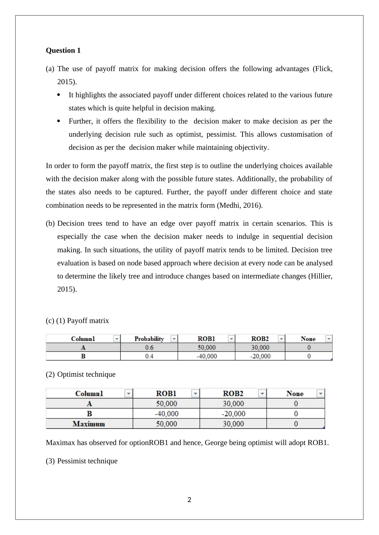
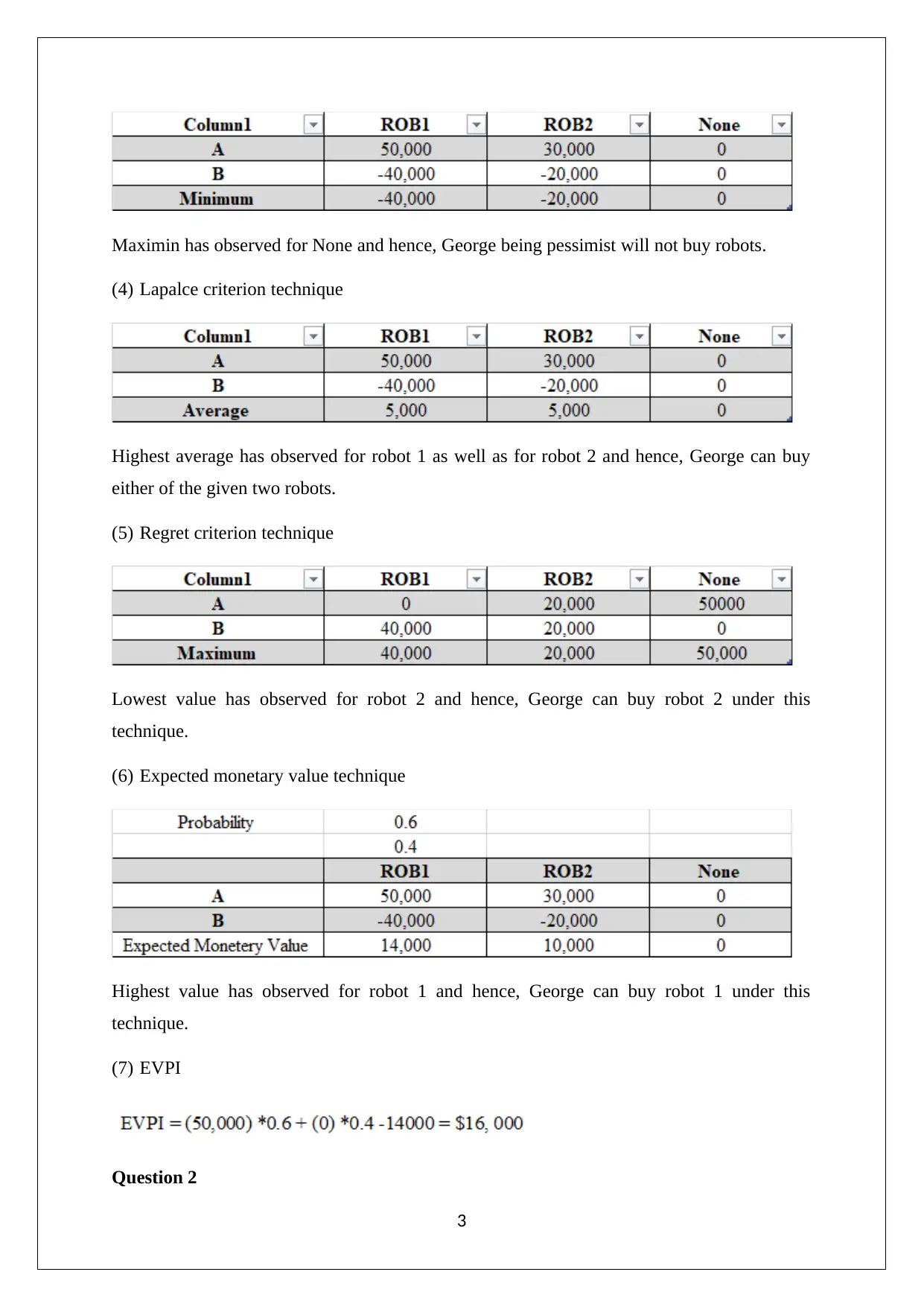
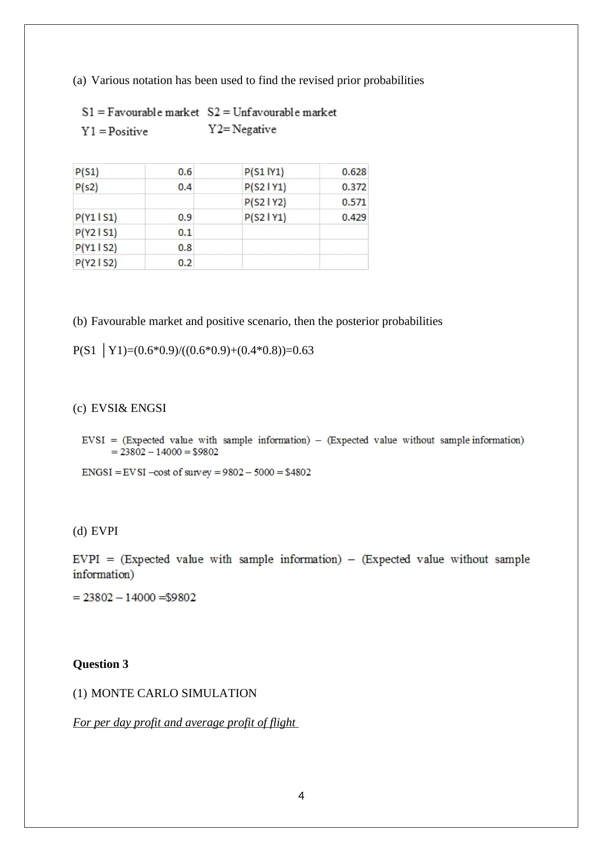
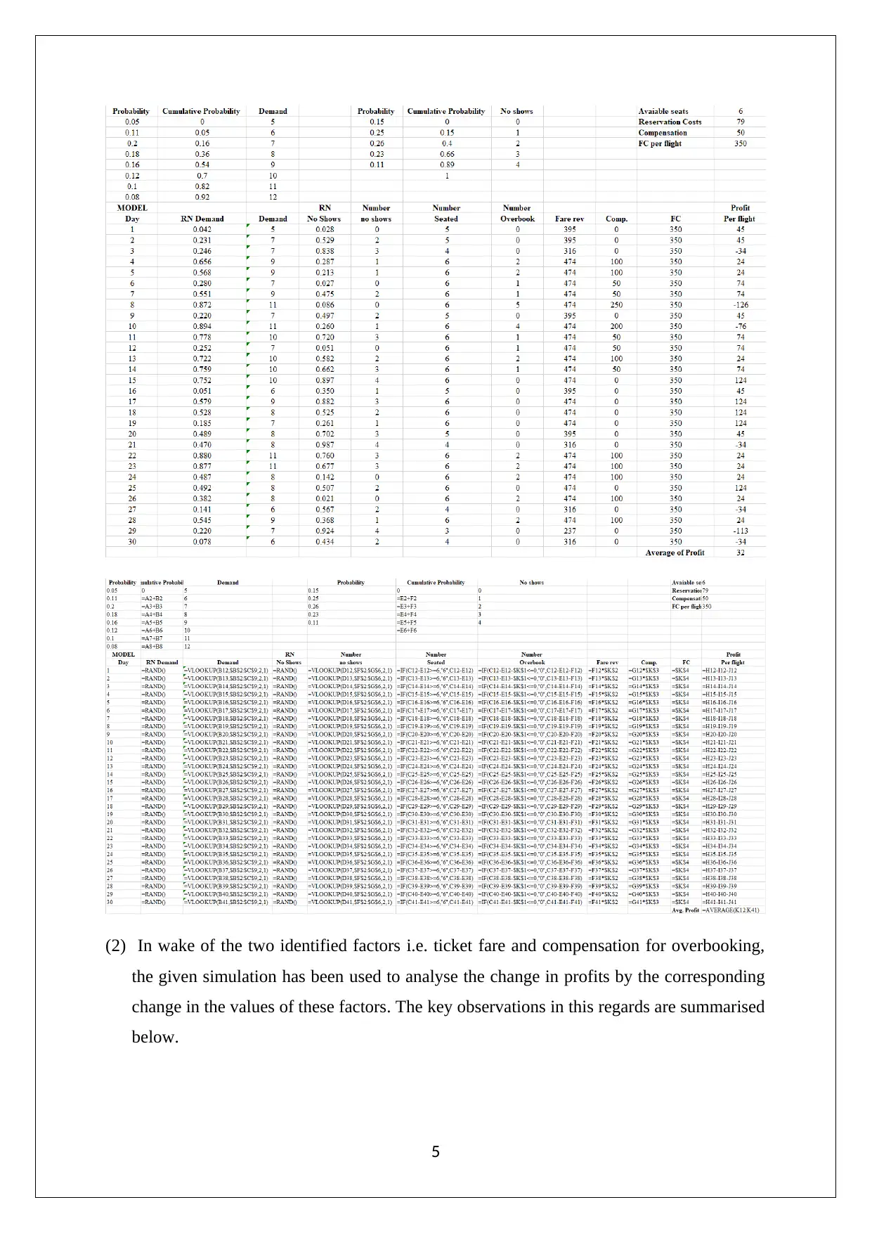
This assignment solution addresses key concepts in decision support tools. It begins with an analysis of payoff matrices, outlining their advantages and the steps involved in their development, as well as comparing them with decision trees. The solution then presents a practical application of these tools through a case study involving industrial robots, constructing a payoff matrix and applying different decision-making techniques like Maximax, Maximin, and Expected Monetary Value. The assignment further explores the use of various notations to determine posterior probabilities. It then delves into Monte Carlo simulation, analyzing the impact of ticket fares and overbooking compensation on profits. The solution also includes regression analysis, comparing different models and their predictive power, followed by a break-even analysis for product profitability. The solution includes detailed calculations and references to support its findings, providing a comprehensive understanding of decision-making tools.

DECISION SUPPORT TOOL
STUDENT ID:
[Pick the date]

Question 1
(a) The use of payoff matrix for making decision offers the following advantages (Flick,
2015).
 It highlights the associated payoff under different choices related to the various future
states which is quite helpful in decision making.
 Further, it offers the flexibility to the decision maker to make decision as per the
underlying decision rule such as optimist, pessimist. This allows customisation of
decision as per the decision maker while maintaining objectivity.
In order to form the payoff matrix, the first step is to outline the underlying choices available
with the decision maker along with the possible future states. Additionally, the probability of
the states also needs to be captured. Further, the payoff under different choice and state
combination needs to be represented in the matrix form (Medhi, 2016).
(b) Decision trees tend to have an edge over payoff matrix in certain scenarios. This is
especially the case when the decision maker needs to indulge in sequential decision
making. In such situations, the utility of payoff matrix tends to be limited. Decision tree
evaluation is based on node based approach where decision at every node can be analysed
to determine the likely tree and introduce changes based on intermediate changes (Hillier,
2015).
(c) (1) Payoff matrix
(2) Optimist technique
Maximax has observed for optionROB1 and hence, George being optimist will adopt ROB1.
(3) Pessimist technique
2

Maximin has observed for None and hence, George being pessimist will not buy robots.
(4) Lapalce criterion technique
Highest average has observed for robot 1 as well as for robot 2 and hence, George can buy
either of the given two robots.
(5) Regret criterion technique
Lowest value has observed for robot 2 and hence, George can buy robot 2 under this
technique.
(6) Expected monetary value technique
Highest value has observed for robot 1 and hence, George can buy robot 1 under this
technique.
(7) EVPI
Question 2
3

(a) Various notation has been used to find the revised prior probabilities
(b) Favourable market and positive scenario, then the posterior probabilities
P(S1 │Y1)=(0.6*0.9)/((0.6*0.9)+(0.4*0.8))=0.63
(c) EVSI& ENGSI
(d) EVPI
Question 3
(1) MONTE CARLO SIMULATION
For per day profit and average profit of flight
4

(2) In wake of the two identified factors i.e. ticket fare and compensation for overbooking,
the given simulation has been used to analyse the change in profits by the corresponding
change in the values of these factors. The key observations in this regards are summarised
below.
5

 If there is increase in the ticket fare, then a positive impact on the profits is seen. This
is no surprising considering that higher ticket fare would have positive contribution on
revenues assuming minimal or no impact on demand.
 The overbooking compensation would aid the profits if it is reduced from the current
level as it would lower the expenses incurred in the form of compensation.
It is noteworthy that the above conclusions have been derived based on the simulation model
but the actual result would vary based on the change in the demand & no show schedule
which would be a function of ticket fare and compensation for overbooking.
(3) The Manager
15th May, 2019
Dear Sir
With reference to the changes in the identified variables, it is noteworthy that profits may get
improved but detailed analysis needs to be done. This is imperative as higher price would
have adverse impact on demand and hence lower the overbooking. While this may ensure
minimal impact on the occupancy, but the increased revenue to some extent may be
neutralised owing to the decrease in overbooking and lowering revenues from no show of
passengers. The current simulation model does not consider these changes and thereby it is
preferable that requisite pilot about the changes proposed above may be carried out. This
would provide a more accurate insight into the precise impact of alteration in the two key
variables i.e. ticket fare and compensation for overbooking. Suitable changes should be
introduced only after suitable pilot runs have been arranged and reported data analysed.
Yours Faithfully
STUDENT NAME
Question 4
(1) Three regression analysis
6

The significance of the slope would determine if the underlying model is statistically
significant or not. A key input required is p value which for the given model does not exceed
the significance level (0.05), The significance of the given linear regression model is thereby
confirmed (Taylor & Cihon, 2014).
The significance of the slope would determine if the underlying model is statistically
significant or not. A key input required is p value which for the given model does not exceed
7

the significance level (0.05), The significance of the given linear regression model is thereby
confirmed (Lieberman, Nag, Hiller & Basu, 2015).
Unlike the above two models, the given model is a multiple linear regression. The
significance of the relationship between the dependent and independent variables can be
ascertained using the ANOVA table. The key parameter of interest is significance F value
(0.0048) . Owing to this value not exceeding significance of level (0.05), hence it can be
claimed that the given multiple regression is significant in statistical terms (Hillier, 2016).
(2) From the above discussion, a key point is that in Model 1, the GMAT slope coefficient is
significant. Similarly, in Model 2, the AGE slope coefficient is significant. Model 1 does not
include AGE as an independent variable. Model 2 does not include GMAT as an independent
variable. However, Model 3 includes both the independent variables and thereby has a higher
predictive power which is captured by the higher coefficient of determination that the simple
regression models. Hence, Model 3 is the most superior model (Lind, Marchal &Wathen,
2016).
(3) Prediction of GPA score
8

Question 5
(1) The break-even units for product A
Units = FC / (Selling price per unit –VCper unit)
= 1200 / (12 – 6) = 200
Now,
Beak-even ($) = Total beak-even units * Selling price per unit
= 200 * 12 = $2400
(2) Units for generating $600 profit and the corresponding margin of safety
Units = (Profit + FC) / (Selling price per unit –VCper unit)
= (600+1200) / (12-6) = 300
Margin of safety = Selling price per unit{(Units)– (Break-even units)}
= 12 {300-200} = $1200
(3) Given units = 250
Gross profit (Revenue) = Given units * (Selling price per unit –VC per unit)
= 250 * (12 – 6) = $1500
Net profit = Revenue – FC
= $1500 - $1200
=$300
9

(4) Product A would have 2 N units and product B would have N units.
The unit contribution margin B = selling price – VC = 20-8 = $12
Profit (Before tax) = Profit (After Tax) / (1- Tax Rate) = 1400/ (0.70) = $2000
Gross profit of A = 12 N
Gross profit of B = 12 N
Gross profit of A & B Jointly= 24 X
FC = Gross profit of A & B Jointly– Profit (Before tax)
5200 = 24N – 2000 and thus, N = 300
Therefore,
There will be 2N= 600 units of A and N = 300 units of B. Further, there would be 600*12 =
$7200 of A and 300*20 = $6000 of B.
10

References
Flick, U. (2015). Introducing research methodology: A beginner's guide to doing a research
project (4thed.). New York: Sage Publications.
Hillier, F. (2016).Introduction to Operations Research.(6thed.). New York: McGraw Hill
Publications.
Lieberman, F. J., Nag, B., Hiller, F.S. & Basu, P. (2015).Introduction To Operations
Research (5thed.).New Delhi: Tata McGraw Hill Publishers.
Lind, A.D., Marchal, G.W. &Wathen, A.S. (2016).Statistical Techniques in Business and
Economics (15thed.). New York : McGraw-Hill/Irwin.
Medhi, J. (2016). Statistical Methods: An Introductory Text (4thed.). Sydney: New Age
International.
Taylor, K. J. & Cihon, C. (2014).Statistical Techniques for Data Analysis (2nded.).
Melbourne: CRC Press.
11